Week 3 - Solving second order ODEs

AIM: write a program in MATLAB to solve second order ODE of motion of simple pendulum with dampind.

OBJECTIVE:

1. To write a program to simulate the transient behavior simple pendulum.
2. TO create a animation of the motion of simple pendulum.

THEORY:

ORDINARY DIFFERANTIAL EQUATION(ODE): An ordinary differential equation (also abbreviated as ODE), in Mathematics, is an equation which consists of one or more functions of one independent variable along with their derivatives. A differential equation is an equation that contains a function with one or more derivatives.

SIMPLE PENDULUM :

A simple pendulum is defined to be an object that as a small mass and also known as a bob ,which is suspended from a light wire or string. as shown in figure.

SIMPLE PENDULUM

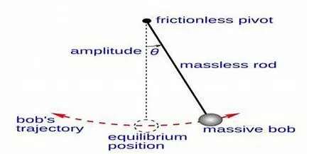
the dynamic behavior of a simple pendulum bob to understand its motion when the pendulum starts its motion at initial push at rest.it express force side ways.It displase it from equilibrium possition to starts to occilates the pivot point it swing back ond forth genarally simple pendulum is casidered as a simple hormonic motion(SHM)and is given equation.

`d^2theta/dt^2+g/lsintheta=0`

Where,

θ">θ = angular displacement of the pendulum bob;

g = acceleration due to gravity in m/s²;

l">l = length of the pendulum in m.

once a pendulum is set into a ossilation it ossilation decrease over a period of time and eventially comes to rest but there ,is observed the time period of vibrating and frequency remains the same ,there such type is damped vibration. the equestion as follows.

`frac{d theta}{dt}=frac{d theta1}{dt}=theta2`

`frac{d^2theta}{dt}=frac{d^2theta1}{dt}=frac{d}{dt}(frac{d theta1}{dt})=frac{d theta2}{dt}`

substitute this in the second order ODE for a simple pendulum,we get ,

`frac{d^2 theta}{dt^2}+frac{b}{m}(frac{d theta }{dt})+frac{g}{l}sin theta =0`

`frac{d^2 theta}{dt^2}+frac{b}{m}(frac{d theta1}{dt})+frac{g}{l}sintheta1=0`

`frac{d^2 theta2}{dt^2}+frac{b}{m} theta2+frac{g}{l}sin theta1=o`

this is a first order differantial equestion, hence can write ,

`therefore frac{d theta1}{dt}=theta2`

`therefore frac{d theta2}{dt}=-frac{b}{m} theta2-frac{g}{l}sintheta2`

writing the equestion in the form of matric .

`frac{d}{dt}[theta1,theta2]= [theta2, -frac{b}{m}theta2-frac{g}{l}sintheta1]`

where,

θ1">θ1= Angular Displacement of the pendulum bob;

θ2">θ2= Angular Velocity of the pendulum bob.

By solving the above equation in Matlab, we can get the values of angular displacement and angular velocity with respect to time.

MATLAB PROGRAM:The values of length of the pendulum 'l">l' is taken as 1 m, mass of the pendulum bob ‘m’ is taken as 1 kg and damping coefficient ‘b’ is taken as 0.05. The motion of simple pendulum is simulated between 0-20 sec, for angular displacement 'θ1">θ1' = 0, angular velocity 'θ2">θ2θ2' = 5 rad/sec at time t=0.

clear all
close all
clc

%inputs

%damping coefficiant
b = 0.05;
%acceleration due to gravity
g = 9.81;
%length of string
l = 1;
%mass of the bob
m = 1;

%initial condition

theta_0 = [0;3];

%time points

t_span = linspace(0,20,500);

%solveing ODE
[t,results] = ode45(@(t,theta)ode_function(t,theta,b,g,l,m),t_span,theta_0);

%Plotting Angular displacement and Angular velocity w.r.t Time
plot(t,results(:,1),'linewidth',3);
hold on
plot(t,results(:,2),'linewidth',3);
axis([0 20 -4 4]);
xlabel('time-(sec)');
ylabel('Angular displacement and Angular velocity');
grid on
title('Damping Effect in Simple Pendulum');

%Animation of Pendulum
%Counter Variable = ct
ct=1;
theta = results(:,1);
for i=1:length(theta)
theta1=theta(i);
x0=0;
y0=0;
x1=1*sin(theta1);
y1=-1*cos(theta1);

figure(2)
title('Motion of Simple Pendulum');
plot([-1 1],[0,0],'linewidth',8,'color','b');
hold on
plot([x0 x1],[y0 y1],'linewidth',5,'color','r');
hold on
plot(x0,y0,'H','markersize',10,'MarkerEdgeColor','g','MarkerFaceColor','r');
plot(x1,y1,'O','markersize',30,'MarkerEdgeColor','r','MarkerFaceColor','g');
grid on;
axis([-1.5 1.5 -1.5 0.5]);
pause(0.01);
hold off;
M(ct) = getframe(gcf);
ct=ct+1;

end
%Making the animation by collecting each frame
movie(M)
videofile = VideoWriter('pendulum.avi','uncompressed AVI');
open(videofile);
writeVideo(videofile,M);
close(videofile);

1. The code strts with clear all, close all, clc. clear all is clear the data stored in work space ,close all is a cammand that close the plots and figures,clc cammond is used to clear the commond window.
2. The inputs is given as follows b,g,l and m . angular displacement `theta1=0`and angular velocity`theta2=5rad-sec`.
3. the time span of pendulum is taken t_span is 20seconds and 500 interwalls.
4. To establish the relation between all the input values in second order ODE, a different function code is written which is as follows,

   function [dtheta_dt] = ode_func(t,theta,b,g,l,m)
   
   theta1 = theta(1);
   theta2 = theta(2);
   dtheta1_dt = theta2;
   dtheta2_dt = -(b/m)*theta2 - (g/l)*sin(theta1);
   dtheta_dt = [dtheta1_dt; dtheta2_dt];
   end

5. The function code is derived as the LHS of first value is theta 1 and second value is theta2.
6. All corresponding equestion is entering in funtion is name as 'ode_func' and the main code of special sytax is 'ode45'.
7. ODE45 is inbuilt matlab function and solve the 2nd ,4thand 5th order to esimate errorrs and determine stepwise.in differential equestion ode45 is more accurate than ode23.
8. After the [t,results] isthe arrey and we needs the plot with time and results(1)is the angular displacement and results(2)is the angular velasity .and plots are created by using plot cammand.
9. By using this result, garph of angular displacement and angular velocty is ploted.
10. Then counter ‘ct’ is initialized. Here ‘ct’ is a variable that simply increments by a specific step value in every iteration of a loop.
11. To provide continuous motion to the pendulum, a ‘for’ loop is used where all the values of ‘t_span’ are assigned to a variable ‘i’ one at a time. The coordinates of the points of line (x0, y0, x1, y1) and their corresponding relations are entered to form the link or string of the pendulum. This line and its motion is thus plotted using suitable axis. The ‘marker’ command is used to form a circle or the bob of the pendulum and the counter is incremented by 1.
12. The ‘pause’ command is used to achieve better animation speed.
13. Then ‘getframe’ command is used to capture the motion of the lines and stored in a variable M.
14. By using ‘movie’ command, Matlab is going to make a movie with all the frames stored in variable M
15. To save this movie, the ‘videofile’ command is used which has the option to store the video in an Uncompressed ‘avi’ format along with the file name.
16. Then the video file is opened after the plot, the movie is run and after completion the video stops or closes.

PROGRAM OUTPUT:

RESULTS: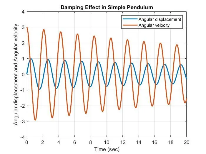

In above ploted graph the red color represents the angular velosity and blue represents the displacement.with respect to time the time is from 0to 3 and 500 values.

ERRORS:

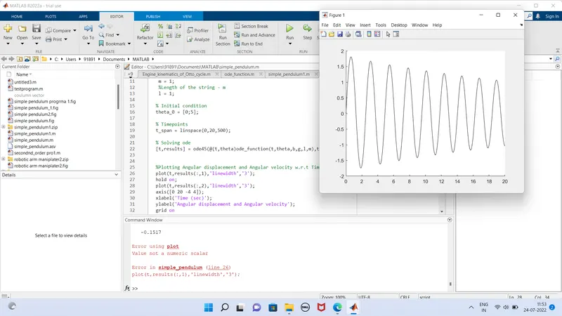
error: in this error im using single qouted in plot(t,results(:,1),'linewidth','3');

animated video: