Week 3 - Solving second order ODEs
2nd Order Differential Equation (Simple Pendulum)
In Engineering, ODE is used to describe the transient behavior of a system. A simple example is a pendulum.
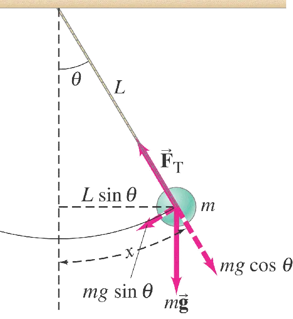
The way the pendulum moves depends on Newton's second law. When this law is written down, we get a second-order Ordinary Differential Equation that describes the position of the "ball" w.r.t time.
Similarly, hundreds of ODEs describe key phenomena, and if we can solve these equations, we will be able to simulate any of these systems.
This ODE represents the equation of motion of a simple pendulum with damping:
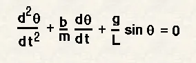
In the above equation,
g = gravity in m/s2,
L = length of the pendulum in m,
m = mass of the ball in kg,
b = damping coefficient.
We are considering the values:
L=1 meter,
m=1 kg,
b=0.05.
g=9.81 m/s2.
Solving the 2nd order differential equation of a Simple Pendulum
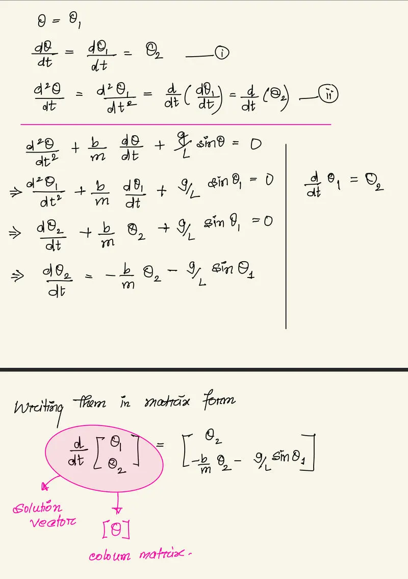
Matlab Code for solving the equation:
Function 'pendulum_2nd_order' Explanation step by step:
%Function Code

function [xdot] = pendulum_2nd_order(t,x) %x represents theta
b = 0.05;
m = 1;
g = 9.81;
L = 1;
xdot = zeros(2,1); %Assigning Null Matrix
xdot(1) = x(2); %First element is angular displacement
xdot(2) = (-b/m)*x(2)-(g/L)*sin(x(1)); %We obtain this after conversion of 2nd order ODE to 1st order ODE

end
First we are writing a function for converting the 2nd order differential equation:
- function [xdot] = pendulum_2nd_order(t,x) %x represents theta
We are defining a function 'pendulum_2nd_order' whose output will be 'xdot'. 'x' here represents θ.
- b = 0.05;
m = 1;
g = 9.81;
L = 1
We define the values for the damping co-efficient, mass, gravitational acceleration, and length respectively as given.
- xdot = zeros(2,1); %Assigning Null Matrix
We then are assigning a 2x1 null matrix to the output initially.
- xdot(1) = x(2); %First element is angular displacement
The first element in the matrix is defined to be the angular displacement
- xdot(2) = (-b/m)*x(2)-(g/L)*sin(x(1)); %We obtain this after conversion of 2nd order ODE to 1st order ODE
The second element in the matrix is the angular velocity
We then are assigning a 2x1 null matrix to the output initially.
- xdot(1) = x(2); %First element is angular displacement
The first element in the matrix is defined to be the angular displacement
-
xdot(2) = (-b/m)*x(2)-(g/L)*sin(x(1)); %We obtain this after conversion of 2nd order ODE to 1st order ODE
end
The second element in the matrix is the angular velocity and we terminate our code by writing 'end'.
Main Code
%%
clear all;
close all;
clc

%%
%Initial Conditions
L = 1;
t = linspace(0,20,150);
x0 = [0 3];

%this below step is for solving differential equation using ode45
[t,x] = ode45('pendulum_2nd_order', t, x0);

%%
%Plot for tracing of Angular Displacement and Angular Velocity

subplot(2,1,1)
plot(t,x(:,1), 'color', 'b', 'linewidth', 3);
xlabel('time t in sec');
ylabel('Angular Displacement');
grid on
subplot(2,1,2)
hold on;
plot(t,x(:,2), 'color', 'r', 'LineWidth', 3);
xlabel('time t in sec');
ylabel('Angular Velocity');
grid on;

%%Animation
X0 = 0;
Y0 = 0;

ct = 1; %counter represents frames

for i = 1:length(t)
    X1 = L*sin(x(i,1));
    Y1 = -L*cos(x(i,1));

    figure(2)
    plot([-1 1], [0 0], 'linewidth', 6, 'color', 'g');
    axis([-2 2 -2 2]);
    line([X0 X1], [Y0 Y1], 'linewidth', 2, 'color', 'b');
    hold on;
    plot(X0, Y0, 'O', 'markersize', 3, 'markerfacecolor', 'y');
    plot(X1, Y1, 'O', 'markersize', 20, 'markerfacecolor', 'r');
    title('Damping of Simple Pendulum');
    legend('Support Rod', 'length of pendulum', 'Fixed Point', 'Bod of Pendulum');
    grid on;
    hold off;
    M(ct) = getframe(gcf);
    ct = ct + 1;
end

movie(M)
videofile = VideoWriter('E:\Matlab for Mechanical Engineering\simple_pendulum.avi', 'Uncompressed AVI');
open(videofile);
writeVideo(videofile, M);
close(videofile);
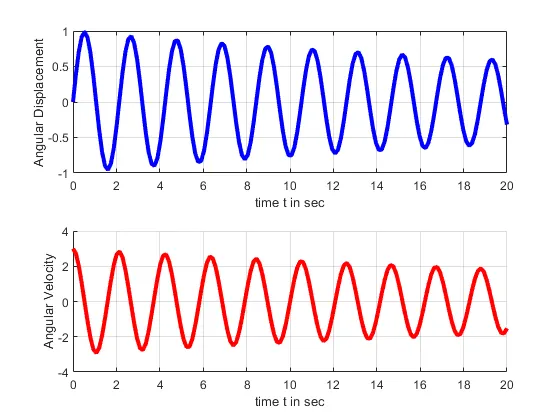
Code Output Screenshots:
A step-by-step explanation of the code:
- %%
clear all;
close all;
clc
We first start by clearing and resetting everything.
- %%
%Initial Conditions
L = 1;
t = linspace(0,20,150);ad
x0 = [0 3];
We then declare the initial conditions. We take an array 't' by using 'linspace' and we take another column array named 'x0'. The first element is initial angular displacement which is set to be 0. And we set the angular velocity to be 3 initially.
- %this below step is for solving differential equation using ode45
[t,x] = ode45('pendulum_2nd_order', t, x0);
We then use the Matlab inbuilt function 'ode45' to solve our equation. In our function named 'pendulum_2nd_order', we converted the 2nd order differential equation to the 1st order differential equation. 'ode45' is solving the 1st order differential equation for us. Here, 't' integrates the system of differential equations for the function with initial conditions x0
- %%
%Plot for tracing of Angular Displacement and Angular Velocity
subplot(2,1,1)
plot(t,x(:,1), 'color', 'b', 'linewidth', 3);
xlabel('time t in sec');
ylabel('Angular Displacement');
grid on
subplot(2,1,2)
hold on;
plot(t,x(:,2), 'color', 'r', 'LineWidth', 3);
xlabel('time t in sec');
ylabel('Angular Velocity');
grid on;
We take two subplots one for the angular displacement and another for the angular velocity. In subplot(2,1,1) we plot the angular displacement. Along the x axis, we take the values for the timespan and along the y axis, we take the values for the theta (x) for the first row which is our angular displacement. We make the color blue with a line width of 3. Along the x-axis, we label it to be 'time t in sec' and along the y axis we label it as 'Angular Displacement'.
In subplot(2,1,2) we plot the angular velocity. Along the x-axis, we take the values for the timespan and along the y axis, we take the values for the theta (x) in the second row which is our angular velocity. We make the color red with a line width of 3. Along the x-axis, we label it to be 'time t in sec' and along the y axis we label it as 'Angular Velocity'.
We turn the grid on for both the cases for better understanding.
Animation Part
- %%Animation
X0 = 0;
Y0 = 0;
We take x and y origin coordinates to be at the zero position.
- ct = 1; %counter represents frames
We take counter for our convenience. It will help us store each frame separately which we in the end can collect together to make our desired simulation of a simple pendulum.
- for i = 1:length(t)
X1 = L*sin(x(i,1));
Y1 = -L*cos(x(i,1));
figure(2)
plot([-1 1], [0 0], 'linewidth', 6, 'color', 'g');
axis([-2 2 -2 2]);
line([X0 X1], [Y0 Y1], 'linewidth', 2, 'color', 'b');
hold on;
plot(X0, Y0, 'O', 'markersize', 3, 'markerfacecolor', 'y');
plot(X1, Y1, 'O', 'markersize', 20, 'markerfacecolor', 'r');
title('Damping of Simple Pendulum');
legend('Support Rod', 'length of pendulum', 'Fixed Point', 'Bod of Pendulum');
grid on;
hold off;
M(ct) = getframe(gcf);
ct = ct + 1;
end
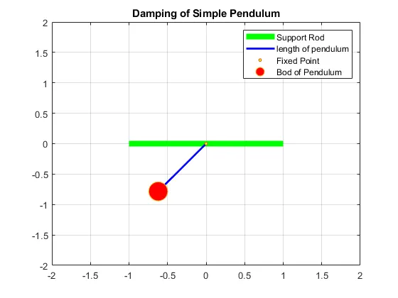
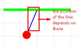
We take a for loop to iterate our frames for generating the animation. The position of the pendulum depends on the value of the theta. The x coordinate of the pendulum will be X0 and sine of the length of the pendulum. The y coordinate of the pendulum will be Y0 and the cosine of the length of the pendulum.
We hold on to the figure and turn it off after recording one frame in the iteration.
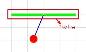
We create a line by plotting the x coordinates (-1, 1) and y coordinates (0, 0).
We then take the axis with x and y coordinates from -2 to 2.
We then put two circle marks one of size 3 colored yellow and another of size 20 with the color red.
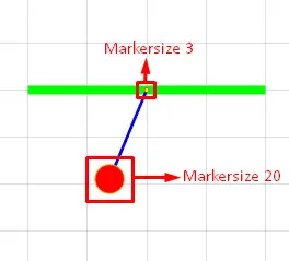
We then title it to be 'Damping of Simple pendulum'.
We use four legends for a better understanding of the figure.
We turn the grid on for better position understanding.
We use the 'getframe' command in order to get each frame per iteration and save it to M(ct).
We add 1 to the counter after each frame is stored and terminate loop by 'end'.
Creating the animation:
- movie(M)
videofile = VideoWriter('E:\Matlab for Mechanical Engineering\simple_pendulum.avi', 'Uncompressed AVI');
open(videofile);
writeVideo(videofile, M);
close(videofile);
We use the 'movie' command in order to create a movie/animation. We create an animation from the collected frames of M added by each counter. We use the 'VideoWriter' command to save it in our desired location and declare it to be 'a videofile'. We open the video file and store the animation created by the 'movie' command of the frames generated during individual iterations of them for a loop by using 'writeVideo' command. After it is done we close the videofile. Thus our simulation for the pendulum is created.
The link for the video is given below: