Week 3 - Solving second order ODEs

% A function program which will be called in the main program to solve the
% ODE


function [dtheta_dt] = ode_func(t,theta,b,g,l,m)

theta1= theta(1);
theta2= theta(2);
dtheta1_dt = theta2;
dtheta2_dt = -(b/m)*theta2 - (g/l)*sin(theta1);
dtheta_dt = [dtheta1_dt; dtheta2_dt];
end 


% Objective: Solving second order ODEs of a penedulum


clear all
close all
clc


b = 0.05; % damping coefficient
g = 9.81; % gravity (m/s^2)
l = 1;  % length of the spring (m)
m = 0.1;  % mass of the bob (kg)

% initial condition
% angular displacement is 0 and angular velocity is 5

theta_0 = [0;5];

% time span
% Pendulum oscillates between 0-20 seconds

t_span = linspace(0,20,600);

% solving ODE
[t,results] = ode45(@(t,theta) ode_func(t, theta, b,g,l,m), t_span, theta_0);

%Plotting
figure(1)
hold on
plot(t,results(:,1))
plot(t,results(:,2))
title('Damped Harmonic motion of a Pendulum')
legend('Angular displacement', 'Angular velocity')
ylabel('Plot')
xlabel('Time(seconds)')



% For loop 
% Before starting the for loop, a counter value was defined

ct =1;
 for i = 1:length(results(:,1))
 x_start = 0;     
 y_start = 0;
 x_end = l*sin(results(i,1));
 y_end = -l*cos(results(i,1));
 
 % plotting the animation
 figure(2)
 plot([-1 1], [0 0], 'linewidth', 5)
 hold on
 plot([x_start x_end],[y_start y_end],'linewidth',3)
 hold on
 
 plot(x_end,y_end,'o','markersize',20,'markerFacecolor','y')
 title('Animation of transient behaviour of a Pendulum')
 axis([-1.5 1.5 -1.5 1])
 pause(0.03)
 hold off 
 
 M(ct) = getframe(gcf);
 ct = ct+1;
 
 end


% Animation of the pendulum

 movie(M)
videofile=VideoWriter('Pendulum Animation.avi', 'uncompressed avi');
open(videofile)
writeVideo(videofile,M)
close(videofile)
 





 

Explanation of Code :-

Step_1 :-

-> To solve a 2nd order ODE, we are creating a function.

-> In this function we are converting 2nd order ODE into 1st order ODE to get two results and assigning them into an array dtheta_dt.

-> IN order to covert we taking theta _1 = theta(1), theta_2 as theta(2).

Step_2 :-

-> Now we are writing the main code to solve the 2nd order ode.

-> In this step we are giving the inputs and initial conditions provided in the question.

-> Also taking the time span of pendulum oscillations up to 20sec for 500 values.

Step_3 :-

-> Writing ode45 syntax

• Ode45 was used, it is a function in Matlab that solves ordinary or partial differential equations using a numerical method.
• The function ode45 takes 3 inputs. The 3 inputs are the function to be integrated, the time span and the initial conditions. [t, results] means that the results that have been calculated with respect to time.

Step_4 :-

-> Plotting the results in a single figure using hold on command. And labeling the plot.

Step_5 :-

-> Creating an animation to demonstrate simple pendulum using for loop and get frame.

A for loop is a repetition control structure that allows you to efficiently write a loop that needs to execute a specific number of times. a counter loop was added before the For loop. the start and endpoints for x and y-axis have been defined. The loop is used where all the values of timespan are assigned to a variable 'i' one at a time. The coordinates of [ xo x1 y0 y1] and their corresponding relations are entered to form a 'string' of the pendulum.

-> taking theta_2 = results(:,1), giving ct = 1;

-> Creating a for loop and taking i = length(theta2).

-> Assigning theta2(i) to THETA1.

-> giving the initial values x0 = 0; y0 = 0;

-> and taking the end point x1 = L*sin(THETA1); y1 = -L*cos(THETA1);

Step_6:-

-> Now we are creating a plot to get the frames.

-> firstly, we are plotting the fixed points and giving hold on command.

-> for the second one we are plotting the length of the rod.

-> for the third one we are creating a plot to make a circular anime using marker command which is considered as weight connected to the rod.

-> Now setting the axis using axis command and giving a pause limit of 0.003.

-> Creating the movie frame using getframe command and giving ct = ct+1, ending the for loop.

Step_7 :-

-> After the plot is converted into frames now, we are creating it into a movie(M).

-> Creating a video file by writing it as simple_pendulum.avi which is uncompressed avi.

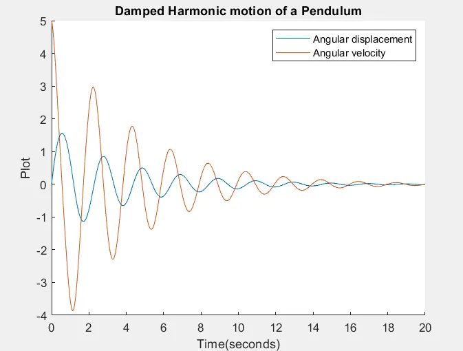
PLOT:

After calculating the results, a graph has to be plotted, the graph contained two plots.

One for angular displacement with respect to time and one for angular velocity with respect for time.

ANIMATION: The link for the animation is:

https://drive.google.com/file/d/1FxmszKXKPy1AIB5p7wWtzkYbXua4_-iv/view?usp=sharing

Errors during programming:

The pendulum starts oscillating in an inverted direction in an animated video.

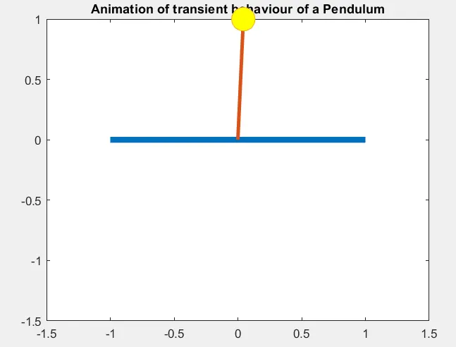
• The step taken to overcome this error:

The final co-ordinate, y_end = 1*cos(theta_2 ) changed to y_end = -1*cos(theta_2 )

Conclusion:

The simulation of the transient behavior of a simple pendulum is successfully created by using a program in MATLAB.