Week 3 - Solving second order ODEs

Aim: To Write a program in Matlab\Octave that will simulate the pendulum motion, just like the one shown in the start of this challenge.

Theory:

Pendulams have many uses and were utilized even before the digital age. They are used in clocks and metronomes due to the regularity of their period, in wrecking balls and playground swings, due to their simple way of building up and keeping energy.

A simple pendulam consists of a point mass or ball suspended on a string or wire that has negligible mass. The simple pendulum is another mechanical system that moves in an oscillatory motion. It consists of a point mass m suspended by means of light inextensible string of length l from a fixed support. The motion occurs in a vertical plane and is driven by a gravitational force.

In the figure the forces which are acting on the mass are shown. The tangential force of gravitational force always acts towards the mean position which is opposite to the displacement. if the pendulam weight is pulled to a relatively small angle from the vertical and let go, It will swing back and forth at aregular period and frequency. Figure 1 shows a simple pendulam.

figure 1

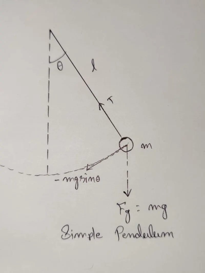
figure 1: simple pendulam

The above figure shows a idealized simple pendulam with a massles string of rod of length l from the mass m. The arc shows the travel path of the mass. If the mass is pulled from its position and let go, it will swing back and forth. The time taken to travel from the farthest right position to the farthest left position and go back to thr farthest right position is called period of the pendulam.

The primary force acting on the mass is gravitational force. In regard there maybe a damping force due to the friction at the pivot and air resistance.

Let s(t) be the distance along the arc from the lowest point to the position of the mass at time t, with displacement to the right considered positive. Let theta(t) be the corresponding angle with respect to the vertical. The figure shows tangential and radial components of the gravitational force on the pendulum mass. The force exerted by the string balances the radial component so that the only relevant force producing the motion is the tangential component of the gravitational force.

Equations used:

The following Ordinary Differential Equation represents the equation of motion of a simple pendulum with damping

(d^2(theta)/dt^2) + b/m(dtheta/dt) + g/L(sin(theta)) = 0

In the above equation,

g = gravity in m/s2,

L = length of the pendulum in m,

m = mass of the ball in kg,

b=damping coefficient.

theta = theta1

dtheta/dt = dtheta1/dt = theta2 ....(i)

d^2theta/dt^2 = dtheta1^2/dt^2 = d/dt(dtheta1/dt) = d/dt(theta2) ...............(i)

d^2theta/dt^2 + b/m dtheta/dt + g/L sintheta = 0

d^2theta1/dt^2 + b/m dtheta1/dt + g/L sintheta1 = 0

dtheta2/dt + b/m theta2 + g/L sintheta1 = 0

dtheta2/dt = -b/m theta2 - g/L sintheta1

d/dt [theta1;theta2] = [theta2; -b/m theta2 - g/L sin theta1]

d/dt [theta1;theta2] is considered as solution vector.

code 1:

clear all
close all
clc

b = 0.05  % damping coefficient
g = 9.81  % gravity
l = 0.1     % length of string
m = 0.1  % mass of the ball

% initial condition
% angular displacement 0, angular velocity 3
theta_0 = [0;5]

% time points
t_span = linspace(0,20,500)

% solve ODE
[t, result] = ode45(@(t,theta) ode_func(t, theta, b, g, l, m),t_span,theta_0)

% plotting
plot(t, result(:,1))
hold on
plot(t, result(:,2))
xlabel('time')
ylabel('velocity and dispacement')

Output :

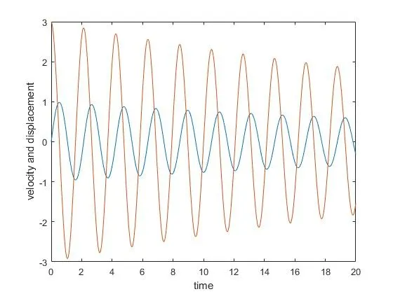
Output Plot:

Explanation:

Before writing the code, it's important to start with clear all, close all and clc commands

Clear all - removes data from the workspace, freeing up system memory

Close all- deletes the current figure or the specified figure

clc - clears all input and output from the Command Window display, giving you a "clean screen

Next the inputs and variables are defined. The damping coefficient, gravity, length of the spring and mass of the ball all have been defined.

Next the initial conditions, the angular displacement and angular velocity have been defined. Time span has also been defined.

Next to solve the ODE a function ode45 is used. It is a function in matlab that solves ordinary pertial differential equations using numerical method.

After calculating the results, a graph is plotted, the graph contained two plots. One for angular displacement with respect to time and one for angular velocity with respect for time. The graph is labeled as 'time' in x direction and 'velocity and displacement' in y direction.

function code:

function [dtheta_dt] = ode_func(t,theta,b,g,l,m)
theta1 = theta(1)
theta2 = theta(2)
dtheta1_dt = theta2
dtheta2_dt = -(b/m)*theta2-(g/l)*sin(theta1)
dtheta_dt = [dtheta1_dt; dtheta2_dt]
end

Explanation:

Taking dtheta_dt as an array with an function name ode_func with values of t for time, theta, b for damping coefficient g for gravity, l for length of string amd m is for mass of the ball. Since theta1 and theta2 are considered as solution vector hence, theta1 will be the 1st value of solution vector theta which is theta(1). Similarly, theta2 will be 2nd value of solution vector theta which is theta(2). Then theta2 is defined (equation (i) ). Then equation (iii) is added. And then dtheta_dt is expressed in a 2x1 matrix of dtheta1_dt and dtheta2_dt elements.

Final Code:

clear all
close all
clc

b = 0.05  % damping coefficient
g = 9.81  % gravity
l = 1     % length of string
m = 1  % mass of the ball

% initial condition
% angular displacement 0, angular velocity 3
theta_0 = [0;3]

% time points  pendulum oscillates between 0 = 20 sec.
t_span = linspace(0,20,500)

% solve ODE
[t, result] = ode45(@(t,theta) ode_func(t, theta, b, g, l, m),t_span,theta_0)

% plotting
plot(t, result(:,1));
hold on
plot(t, result(:,2));
xlabel('time');
ylabel('velocity and displacement');

% for loop
% a counter is placed before the loop

    ct = 1
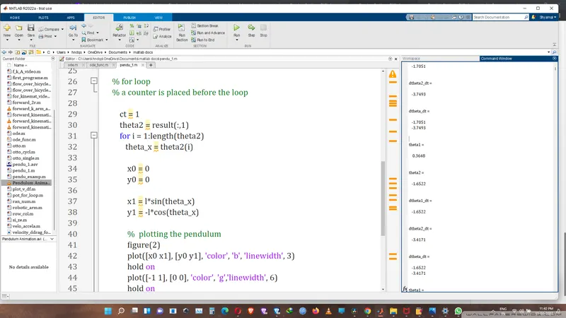
    theta2 = result(:,1)
    for i = 1:length(theta2)
       theta_x = theta2(i)

        x0 = 0
        y0 = 0

        x1 = l*sin(theta_x)
        y1 = -l*cos(theta_x)

        %  plotting the pendulum
        figure(2)
        title('Simple Pendulum')
        plot([x0 x1], [y0 y1], 'color', 'b', 'linewidth', 3)
        hold on
        plot([-1 1], [0 0], 'color', 'g','linewidth', 6)
        hold on
        plot(x1,y1,'o','markers',15,'markerfacecolor','r')
        hold off
        axis([-1.5 1.5 -1.5 0.5])
        pause(0.02)
        
        M(ct) = getframe(gcf)
        ct = ct+1
    end

movie(M)
videofile = VideoWriter('Pendulum Animation','Uncompressed AVI');
open(videofile)
writeVideo(videofile,M)
close(videofile)

Explanation:

Now to create a pendulum animation for loop is used. Usng for loop index at length of theta2, theta_x is defined.

Since the pewndiulum starts from initial position of 0 which is at stable so, x0, y0 will be 0. X1 and y1 will be the poosition of displacement. And it is defined as for x1 = l*sin(theta_x) and y1 = l*cos(theta_x).

Now to plot the pendulum x0, x1 and y0,y1 coordinates are connected (the base of pendulum).

Using hold on command on the same cartesian plane coordinates of pendulum string are connected. And the mass is plotted at one end of the string using marker command. The other end of the string is connected to the base of pendulum.

The hold off command is used to add new plot while retaining old plot. Thats why using hold off command the pendulam mass is added while retaining the pendulam base curve and string.

Then the axis range is defined and the frame interval is set to 0.02 sec.

M is an array. ct coumts all the pendulam movements and getframe(gcf) contains all the frames which are actually the different positions of the ball's movement.

The following command lines are used to create save, open and close the video file of the animation of pendulam ball movement, file name of 'Pendulam Animation'.

movie(M)
videofile = VideoWriter('Pendulum Animation','Uncompressed AVI');
open(videofile)
writeVideo(videofile,M)
close(videofile)

The animation video link is given bellow in the conclusion.

Possible error and prevention:

1. Use of '*' for multiplication is necessary. Otherwise it will lead to error. Using the error notice is a good way to correct these errors.

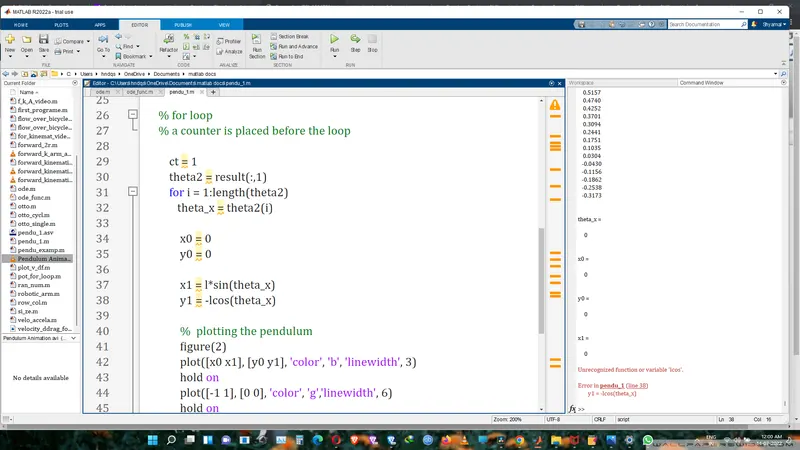
2. Improper use of brackets may resut in conflict. Rechecking is the best way to prevent these mistakes.

Conclusion:

1. The above work can conclude that Matlab can be used for solving the ode of any order mentioned.

2. The animation generated is also supporting the results that we concluded, as the time proceeds the bob slow down and the amplitude of the swing reduces.

3. The link for the animation video file -

https://photos.app.goo.gl/dz6uwx4GWRvLd7wy8