Week 3 - Solving second order ODEs
Aim - The Objective of this challenge is to write a program that can solve the second - order ODE of a simple pendulum and make the animation for the moment of the pendulum in term of angular displacement.
Theory -
Introduction - Many physical problem from fluid mechanics, heat transfer, rigid body dynamics are modeled by second order PDE's. In some probelms fourth order PDE's do aries, however as we split higher order ordinary differential equastions into a system of first order equations.
Problem Statement - Given 2nd order differential equastion -
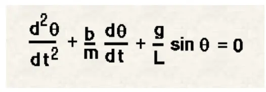
We need to do some assumptions and hand calculation to ghet the 'θ1' and 'θ2'.
d2θ/dt2+b/m (dθ)/dt+g /l sin θ = 0
Converting in to multiple first order equations -
Let's say
θ = θ1
(dθ)/dt = (dθ1)/dt = θ2
d2θ/dt2 = d2θ1/dt2 = d((dθ1)/dt)/dt = dθ2/dt
from all the above equations we simplified the equation as below -
d2θ/dt2+b/m (dθ)/dt+g /l sin θ = 0
In the above equation,
g = gravity in m/s2,
l = length of pendulum in m,
m = mass of the ball in kg,
b = damping coefficient
Given parameters are -
l = 1 m,
m = 1 kg,
b = 0.05
g = 9.81 m/s2,
time (t) = [ 0 -20 ] sec,
angular displacement = 0
angular velocity = 3 rad/s (at t= 0).
ODE's in MATLAB -
An ordinary differential equation (ODE) contains one or more derivatives of a dependent variable, y, with respect to a single independent variable, t, usually referred to as time. The notation used here for representing derivatives of y with respect to t is y′ for a first derivative, y′′ for a second derivative, and so on. The order of the ODE is equal to the highest-order derivative of y that appears in the equation.
For example, this is a second order ODE:
y′′=9y
In an initial value problem, the ODE is solved by starting from an initial state. Using the initial condition, y0, as well as a period of time over which the answer is to be obtained, (t0,tf), the solution is obtained iteratively. At each step the solver applies a particular algorithm to the results of previous steps. At the first such step, the initial condition provides the necessary information that allows the integration to proceed. The final result is that the ODE solver returns a vector of time steps t=[t0,t1,t2,...,tf] as well as the corresponding solution at each step y=[y0,y1,y2,...,yf].
Reference - https://www.mathworks.com/help/matlab/math/choose-an-ode-solver.html
How to create an animation using MATLAB - To create a video from Matlab it have inbuilit commands, we need to follow the process shown below.
clear all
close all
clc

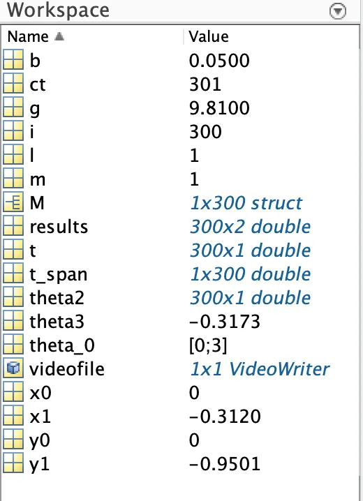
b = 0.05;
g = 9.81;
l = 1;
m = 1;

% initial condition
theta_0 = [0;3];

% time points
t_span = linspace(0,20,300);

% solve ODE
[t, results] = ode45(@(t,theta) ode_func(t,theta,b,g,l,m),t_span,theta_0);
figure (1)
plot(t,results(:,1))
hold on
plot(t,results(:,2))
ylabel('Angular dispalcement Vs Angular velocity')
xlabel('time')
legend('Angular dispalcement Vs Angular velocity')
grid on

figure (2)
plot(results(:,1),results(:,2))
xlabel('position')
ylabel('Angular velocity')
legend('Angular velocity')

theta2 = results(:,1)
ct = 1
for i = 1:length(theta2)
    theta3 = theta2(i)
    %for fixed and moving bar of a pendulam
    x0 = 0
    y0 = 0

    x1 = 1*sin(theta3)
    y1 = -1*cos(theta3)

    %giving axis, color for pendulam
    figure(3)
    plot([-1.1 1.1],[0,0],'LineWidth',3)
    hold on
    plot([x0 x1],[y0 y1],'g','LineWidth',3)
    hold on
    plot (x1,y1,'o','markers',20,'MarkerFaceColor','m')
    xlabel('x-axis')
    ylabel('y-axis')
    hold off
    grid on
    axis([-1.5 1.5 -1.5 0.5])
    % time frame to get video
    pause(0.003)
    M(ct) = getframe(gcf);
    ct = ct+1;
end
% code to run save the video
movie(M)
videofile = VideoWriter('Simple pendulam.avi','Uncompressed AVI');
open(videofile)
writeVideo(videofile,M)
close(videofile)
Suplimentry program to splitting the second order derivative into two parts -
function [dtheta_dt] = ode_func(t,theta,b,g,l,m)

theta1 = theta(1)
theta2 = theta(2)
dtheta1_dt = theta2;
dtheta2_dt = -(b/m)*theta2-(g/l)*sin(theta1);
dtheta_dt = [dtheta1_dt;dtheta2_dt];
end
Error -
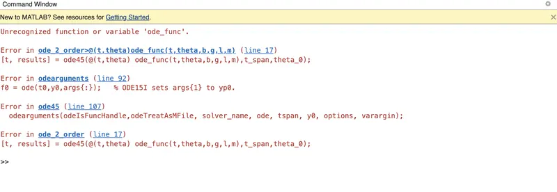
- This Error comes while we create supplimentry program but not saved and using in main program so this error comes.
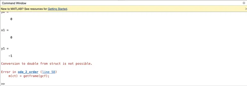
- This error comes while we used 'm' insist of 'M'.
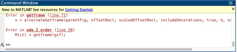
- This error comes while we not played full program video during in 'RUN', so while we complete 'RUN' process and then this error disappeared.
Results -
- Time Vs Angular displacement and Angular velocity -
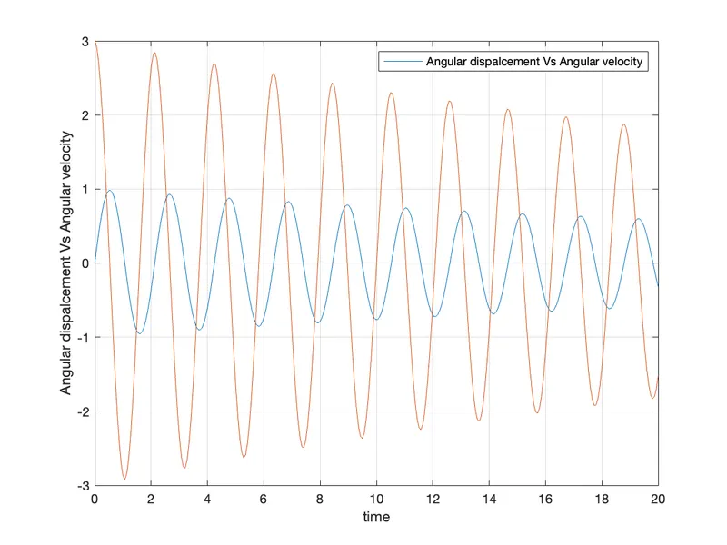
- The plot explains how the angular velocity and angular displacement is varying with respect to time.
- Position Vs Angular Velocity -
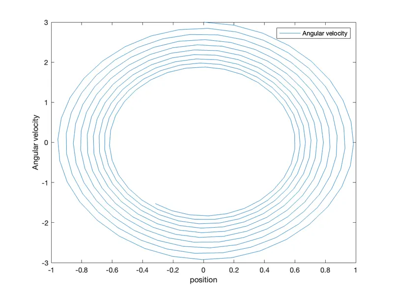
- The plot explains to us the position of the ball on the scale of [-1 1] while it's angular velocity is going to decrease gradually.
- The ball in the simple pendulum starts at a point at a velocity of 3 m/s and as the solution starts, the ball slowly lost it's momentum and made the impression of the path.
- After the given time of 20 sec, the velocity reaches to nearly 1.3 m/s.
- Animation - https://youtu.be/dIkwAmoEMnY