Challenge

Week 3 - Solving second order ODEs

Aim : Code to solve the equation of motion of a simple pendulum with damping and an animation of the motion of the pendulum.

Governing Equations : The equation of motion of a simple pendulum with damping

`(d^2 θ)/(dt^2 )+b/m (dθ)/dt+g/l sinθ=0`

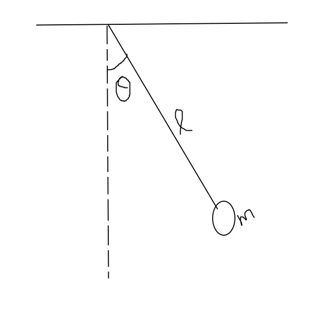
Where

g = gravity in m/s2,

L = length of the pendulum in m,

m = mass of the ball in kg,

b=damping coefficient.

Solving a second order differential equation :

As the given equation is a second order differential equation ,in order to solve that equation we have to create two ODEs,

Let θ=θ1

_{`(dθ)/dt=(dθ1)/dt=θ2`}

_{`(d^2 θ)/(dt^2 )=(d^2 θ1)/dt^2 =d/dt ((dθ1)/dt)=(dθ2)/dt`}

_{`(d^2 θ)/(dt^2 )+b/m (dθ)/dt+g/l sinθ=0`}

_{`(d^2 θ1)/(dt^2 )+b/m (dθ1)/dt+g/l sinθ1=0`}

_{`(dθ2)/dt+b/m θ2+g/l sinθ1=0`}

_{`(dθ2)/dt=-b/m θ2-g/l sinθ1`}

_{`d/dt [(θ1 @ θ1)]=[(θ2 @- b/m θ2-g/l sinθ1)]`}

Let `[■(θ1@θ2)] = θ`

Mathematically Solved the second order differential equation into two ode’s

Code for ode’s in MATLAB :

function[dtheta_dt] = ode_func(t,theta,b,g,l,m)

theta1 = theta(1)

theta2 = theta(2)

dtheta1_dt = theta2;

dtheta2_dt = -(b/m)*theta2-(g/l)*sin(theta1);

dtheta_dt = [dtheta1_dt;dtheta2_dt];

end

explanation : for simplification we first defined the derivatives did by mathematically and used a function command to call the code in main program.

ODE45 is an inbuilt MATLAB command to solve ordinary differential equation(ODE) equations. The syntax is

[x,y] =ode45(@(t,y) fame(t,y),[t0,tend],y0)

x,y : solution vectors, MATLAB returns y for each time of x

Fname. : function that returns dy =F(t,y)

t0,y0. : initial conditions representing y(t0)=y0

tend : final value until which the solution is desired.

code to simulate the pendulum motion :

clear all

close all

clc

b=0.05;

g=9.81;

L=1;

m=1;

 % initial conditions

theta_0 = [0,3];

 
% time points

t_span = linspace(0,20,100);

 
% solve ODE

[t,results] = ode45(@(t,theta) ode_func(t,theta,b,g,L,m),t_span,theta_0);

 

subplot(2,1,1)

plot(t,results(:,1),'linewidth',3)

xlabel('time')

ylabel('angular displacement')

subplot(2,1,2)

hold on

plot(t,results(:,2),'linewidth',3)

ylabel('angular velocity')

xlabel('time')

Explination : in the question it was given the value of L=1 metre, m=1 kg, b=0.05. g=9.81 m/s2. Time span is 0-20 sec, angular displacement=0, angular velocity=3 rad/sec at time t=0. On assigning all the values to the ODE function and plotting we will get the plot as shown in main code with plot screen shot

Subplot is a command used to plot multiple plots in one figure. The syntax is : subplot(number of row, number of column, figure number)

Ex. : subplot (2,1,1) means the figure will divide into two rows and one column and in 1^st row plot will be shown.

Animation code of simple pendulum :

clear all

close all

clc

 
b=0.05;

g=9.81;

l=1;

m=1;

 
% initial conditions

theta_0 = [0,3];

 
% time points

t_span = linspace(0,20,100);

 
% solve ODE

[t,results] = ode45(@(t,theta) ode_func(t,theta,b,g,l,m),t_span,theta_0);

 
subplot(2,1,1)

plot(t,results(:,1),'linewidth',3)

xlabel('time')

ylabel('angular displacement')

subplot(2,1,2)

hold on

plot(t,results(:,2),'linewidth',3)

ylabel('angular velocity')

xlabel('time')


% ANIMATION

 
X0=0

Y0=0

ct=1;

for i=1:length(t)

    X1 = l*sin(results(i,1));

    Y1 = -l*cos(results(i,1));

 
    figure(2)

    plot([-1 1],[0 0],'linewidth',5,'color','g');

    axis([-2 2 -2 2]);

    line([X0 X1],[Y0 Y1],'linewidth',3,'color','b');

    hold on;

    plot(X0,Y0,'o','markersize',3,'markerfacecolor','y')

    plot(X1,Y1,'o','markersize',20,'markerfacecolor','r')

    title('Animation of simple pendulum');

    legend('support rod','length','fixed point','bob')

    grid on;

    hold off

    M(ct)=getframe(gcf)

    ct=ct+1

end

movie(M)

videofile=VideoWriter('simple_pendulum.AVI','uncompressed AVI');

open(videofile)

writeVideo(videofile,M);

close(videofile);

Result : for creating an animation of simple pendulum first define the coordinates for initial point and final point

Let the initial point be x₀ = 0,y₀ = 0 .

final point will be changing with respect to time, so for result we will assign the final points as

X1 = l*sin(results(i,1));

Y1 = -l*cos(results(i,1));

On main code result will change for the value of t given so on assigning our final point to results the final point also changes.

The line I=1:length(t) denotes the value of I changes from 1 to length(t) and each time it stores only one value and executes all the calculations by using the for loop command.

On plotting a figure using initial and final points with respect to time an animation of simple pendulum was formed.

Ct denotes counter. initially ct was assigning with value 1 and by each and every time for loop executes the counter was increased by 1 value by giving the command ct=ct+1

Creating a movie or animation: get individual frames and then save them in an array Called m

I,e., M(ct)=getframe(gcf)

At the end of the for loop if we type movie Matlab is going to create a movie with all those frames

Videowriter is a command used to create video file by giving file name and profile to the video.

Once created the video file we are going open video file by giving the command open(videofile)and then going to write the frames on this video file by using write command

I,e., write(videofile,m) and finally close the video file by using close command I,e., close(videofile)

Error faced while programming:

After coding the programme like this I got an error in movie.

clear all

close all

clc

b=0.05;

g=9.81;

l=1;

m=1;

% initial conditions

theta_0 = [0,3];

% time points

t_span = linspace(0,20,100);

% solve ODE

[t,results] = ode45(@(t,theta) ode_func(t,theta,b,g,l,m),t_span,theta_0);

subplot(2,1,1)

plot(t,results(:,1),'linewidth',3)

xlabel('time')

ylabel('angular displacement')

subplot(2,1,2)

hold on

plot(t,results(:,2),'linewidth',3)

ylabel('angular velocity')

xlabel('time')

% ANIMATION

X0=0

Y0=0

ct=1;

for i=1:length(t)

X1 = l*sin(results(i,1));

Y1 = -l*cos(results(i,1));

figure(2)

plot([-1 1],[0 0],'linewidth',5,'color','g');

axis([-2 2 -2 2]);

line([X0 X1],[Y0 Y1],'linewidth',3,'color','b');

hold on;

plot(X0,Y0,'o','markersize',3,'markerfacecolor','y')

plot(X1,Y1,'o','markersize',20,'markerfacecolor','r')

title('Animation of simple pendulum');

legend('support rod','length','fixed point','bob')

grid on;

hold off

ct=ct+1

M(ct)=getframe(gcf)

end

movie(M)

videofile=VideoWriter('simple_pendulum.AVI','uncompressed AVI');

open(videofile)

writeVideo(videofile,M);

close(videofile);

steps taken to overcome the error:

after replacing the command ct=ct+1 after getframe command my error was rectified and I got the animation of simple pendulum.

clear all

close all

clc

b=0.05;

g=9.81;

l=1;

m=1;

% initial conditions

theta_0 = [0,3];

% time points

t_span = linspace(0,20,100);

% solve ODE

[t,results] = ode45(@(t,theta) ode_func(t,theta,b,g,l,m),t_span,theta_0);

subplot(2,1,1)

plot(t,results(:,1),'linewidth',3)

xlabel('time')

ylabel('angular displacement')

subplot(2,1,2)

hold on

plot(t,results(:,2),'linewidth',3)

ylabel('angular velocity')

xlabel('time')

% ANIMATION

X0=0

Y0=0

ct=1;

for i=1:length(t)

X1 = l*sin(results(i,1));

Y1 = -l*cos(results(i,1));

figure(2)

plot([-1 1],[0 0],'linewidth',5,'color','g');

axis([-2 2 -2 2]);

line([X0 X1],[Y0 Y1],'linewidth',3,'color','b');

hold on;

plot(X0,Y0,'o','markersize',3,'markerfacecolor','y')

plot(X1,Y1,'o','markersize',20,'markerfacecolor','r')

title('Animation of simple pendulum');

legend('support rod','length','fixed point','bob')

grid on;

hold off

M(ct)=getframe(gcf)

ct=ct+1

end

movie(M)

videofile=VideoWriter('simple_pendulum.AVI','uncompressed AVI');

open(videofile)

writeVideo(videofile,M);

close(videofile);

Week 3 - Solving second order ODEs

Ship work like this
in your own course.

Talk to a career counsellor

Ship work like thisin your own course.

Talk to a career counsellor

Ship work like this
in your own course.