Week 3 - Solving second order ODEs

Analysis of simple Pendulum

AIM

To solve simple pendulum and animate the output

Equation

ODE is split into many equation to solve ODE

Equation

`(d^2theta)/(dt^2)+(b/m)(d theta)/dt+g/L sintheta=0`

slit the ODE to solve

`(d theta)/dt=[(d theta_1)/dt,(d theta_2)/dt]`

velocity (1st order ODE)

`(d theta_1)/dt=theta_2`

acceleration (2nd order ODE)

`(d theta_2)/dt=-(b/m)(d theta)/dt-g/L sintheta`

Given Data

length of pendulum

l=1 m

mass

m=1 kg

Damping Co-efficient

b=0.05

gravitational constant

g=9.81 m/s2

simulation time

starting time =0

end time=20 s

number of in-between points

n=150

Python Code

import numpy as np
from scipy.integrate import odeint
import matplotlib.pyplot as plt
import math

#fuction thtat return dz/dt
def model(theta,t,b,g,l,m):

	theta1=theta[0]
	theta2=theta[1]
	dtheta1_dt = theta2
	dtheta2_dt = -(b/m)*theta2 -(g/l)*math.sin(theta1)
	dtheta_dt = [dtheta1_dt,dtheta2_dt]
	return dtheta_dt

b=0.05
g=9.81
l=1
m=1

#initial condition
theta_0=[0,3]

#time loop points
t=np.linspace(0,20,150)

#solve ODE

theta=odeint(model,theta_0,t,args=(b,g,l,m))

#plot result
plt.figure(1)
plt.plot(t,theta[:,0],'b-',label=r'$\frac{d\theta_1}{dt}=\theta2$')
plt.plot(t,theta[:,1],'r--',label=r'$\frac{d\theta_2}{dt}=\frac{b}{m}\theta_2-\frac{g}{L} sin\theta_1$')
plt.ylabel('position')
plt.xlabel('time')
plt.legend(loc='best')
plt.show()

plt.figure(2)
plt.plot(theta[:,0],theta[:,1],'r')
plt.xlabel('velocity')
plt.ylabel('acceleration')
plt.title('Acceleration vs velocity of pendulam')
plt.grid()
plt.show()

#creating count variable
ct=1
# creating Arm movement
for t1 in theta[:,0]:
		#link 1 movement
		x0=0
		y0=0
		#link 2 movement
		x1=(1*math.sin(t1))
		y1=-(1*math.cos(t1))
		

		# creating variable to store image
		filename=str(ct) + '.png'
		ct=ct+1

		#plot Arm movement
		plt.figure()
		#start position
		plt.plot([x0,x1],[y0,y1],linewidth=5,color='k')
		#bob
		plt.plot(x1,y1,'o',markersize=20,color='b')
		plt.plot([-1.5,1.5],[2,2],linewidth=5,color='r')
		plt.xlim([-2.5,2.5])
		plt.ylim([-2.5,2.5])
		plt.title('pendulam animation')
		

		plt.savefig(filename)

Result

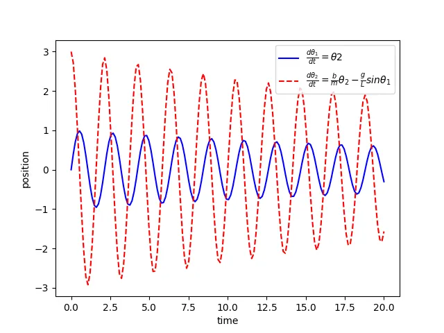
angular displacement, angular velocity result with respect to time

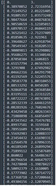
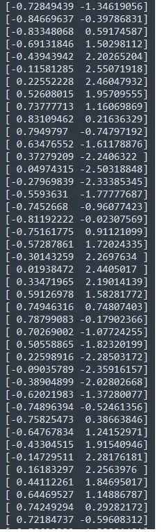
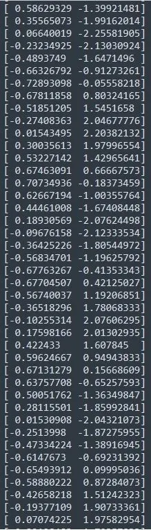
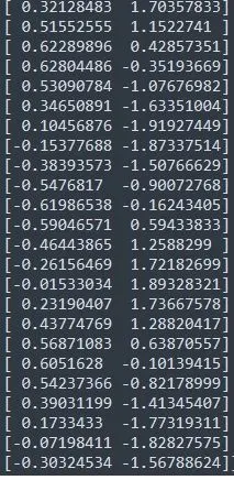
Angular Displacement vs Angular velocity with respected to time and position

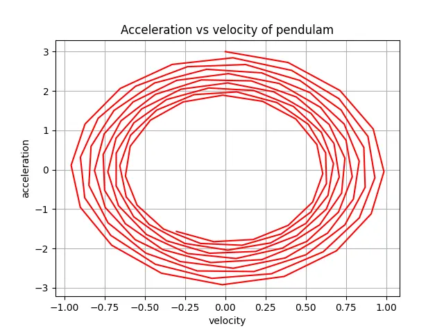
velocity vs Acceleration

pendulum animation

the picture is created using python code and stretched the picture with external software

Result

the pendulum animation is created from the given equation

for a given time and position displacement and velocity are plotted in the graph

displacement vs velocity is a plotted with respect to time