Challenge

Week 3 - Solving second order ODEs

Aim - To solve an ODE and use the calculated information to animate the motion of the pendulum

Introduction-:

In Engineering, ODE is used to describe the transient behavior of a system. A simple example is a pendulum

The way the pendulum moves depends on the Newtons second law. When this law is written down, we get a second order Ordinary Differential Equation that describes the position of the "ball" w.r.t time.

Similarly, there are hundreds of ODEs that describe key phenomena and if you have the ability to solve these equations then you will be able to simulate any of theses systems.

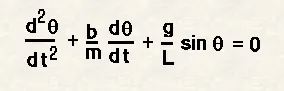
Your objective is to write a program that solves the following ODE. This ODE represents the equation of motion of a simple pendulum with damping.

Asimple pemdulum consits of a point mass suspended on a string oe wire that has negligible mass. When the bob is displaced through some angle pulling the string from its vetical position and is let go,it oscilates back and forth commencing the simple harmonic motion which is given by the following equation.
Calculation:
where-:

b= daming coeficient

m= mass of bob (in kg)

L= length of string (mt)

g= acceleration due to gravity(m/sec^2)

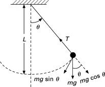
Following is the image of simple pendulum
Code explanation-:

Step 1: Providing the pre requisite values

b = 0.05;
g = 9.81;
l = 1;
m = 0.1;
Step 2: Providing initial conditions
% Initial conditions
theta_0 = [0;5];
In the theta_0 array,'0' is the condition for displacement and '5' is the condition for velocity
%time points
t_span = linspace(0,20,600);
Step 4: Solving the ODE
%solve ode
[t, results] = ode45(@(t,theta) ode_func(t, theta, b,g,l,m),t_span,theta_0);
%plotting
plot(t, results(:,1))
hold on
plot(t, results(:,2))
title('Damping of pendulum harmonic motion')
legend('angular displacement','angular velocity')
ylabel('Plot')
xlabel('time')
ODE45 is the inbuilt command of MATLAB
ODE45 is usually the function of choice among the ODE solvers. It compares methods of orders four and five to estimate error and determine step size. ODE45 is so accurate that its default behavior is to use its interpolant to provide results at intermediate points.
45 in ODE45 stands for the Runge-Kutta(4,5) method. Such method is suited for solving ordinary differential equations by predictions.
ode_func(t, theta, b,g,l,m),t_span,theta_0); i the function which will be used to simulate the motion of pendulums by giving the pre-requisite values
Function Program
function [dtheta_dt] = ode_func(t,theta,b,g,l,m)
theta1 = theta(1);
theta2 = theta(2);
dtheta1_dt = theta2;
dtheta2_dt = -b/m*theta2 - (g/l)*sind(theta1);
dtheta_dt = [dtheta1_dt; dtheta2_dt];
end
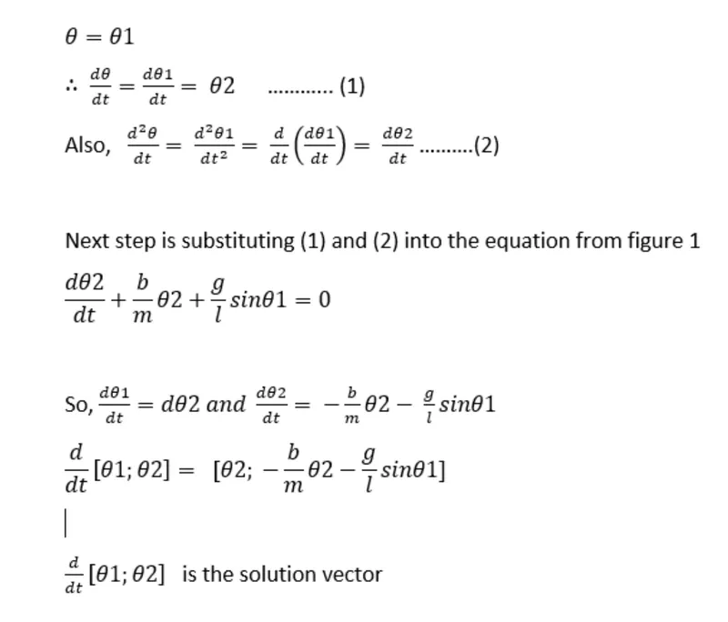
since theta = [ theta(1);theta(2)] is the solution vector
MAIN and final code for solution,plotting and simulation
clear all
close all
clc
%Giving the pre-requisite values for constants in equation
b = 0.05;
g = 9.81;
l = 1;
m = 0.1;
% Initial conditions
theta_0 = [0;5];
%time points
t_span = linspace(0,20,600);
%solve ode
[t, results] = ode45(@(t,theta) ode_func(t, theta, b,g,l,m),t_span,theta_0);
%plotting
plot(t, results(:,1))
hold on
plot(t, results(:,2))
title('Damping of pendulum harmonic motion')
legend('angular displacement','angular velocity')
ylabel('Plot')
xlabel('time')
Part 2 of the code is to establish a for loop for the repetetion control structure,a counter loop was added before the for loop.The start and end points of x and y axis have been defined. The loop is used where all the values of time are assigned to a variable "i" one at a time.
pause command was used to pause the command for a certain period of time(0.03s)
%loop counter
ct =1;
for i = 1:length(results(:,1))
x_start = 0;
y_start = 0;
x_end = l*sin(results(i,1));
y_end = -l*cos(results(i,1));
%plotting animation
figure(2)
plot([0 0],[0 0],'linewidth',4)
hold on
plot([x_start x_end],[y_start y_end],'linewidth',2)
hold on
plot(x_end,y_end,'o','MarkerSize',20,'MarkerFaceColor','auto')
title('Animation of damped oscilation of a simple pendulum')
axis([-1.5 1.5 -1.5 1])
pause(0.03)
hold off
FINAL STEP IS TO CREATE A MOVIE
M(ct) = getframe(gcf);
ct = ct+1;
end
%animation of the motion
movie(M)
videofile=VideoWriter('Pendulum Oscilation.avi', 'uncompressed avi');
open(videofile)
writeVideo(videofile,M)
close(videofile)
RESULTS
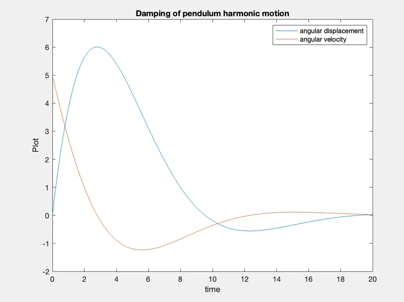
The following figure shows the graph obtained after succesfully compiling and running the solution code
clear all
close all
clc


%Giving the pre-requisite values for constants in equation

b = 0.05;
g = 9.81; 
l = 1;
m = 0.1; 

% Initial conditions
theta_0 = [0;5];

%time points 
t_span = linspace(0,20,600);

%solve ode

[t, results] = ode45(@(t,theta) ode_func(t, theta, b,g,l,m),t_span,theta_0);

%plotting
figure(1)
hold on 
plot(t, results(:,1))
plot(t, results(:,2))
title('Damping of pendulum harmonic motion')
legend('angular displacement','angular velocity')
ylabel('Plot')
xlabel('time')

%loop counter
ct =1; 
for i = 1:length(results(:,1))
    x_start = 0;
    y_start = 0;
    x_end   = l*sin(results(i,1));
    y_end   = -l*cos(results(i,1));

    %plotting animation
    figure(2)
    plot([-1 1],[0 0],'linewidth',4)
    hold on
    plot([x_start x_end],[y_start y_end],'linewidth',2)
    hold on

    plot(x_end,y_end,'o','MarkerSize',20,'MarkerFaceColor','auto')
    title('Animation of damped oscilation of a simple pendulum')
    axis([-1.5 1.5 -1.5 1])
    pause(0.03)
    hold off


    M(ct) = getframe(gcf);
    ct = ct+1;
end

%animation of the motion

movie(M)
videofile=VideoWriter('Pendulum Oscilation.avi', 'uncompressed avi');
open(videofile)
writeVideo(videofile,M)
close(videofile)

Program for function

function [dtheta_dt] = ode_func(~,theta,b,g,l,m)

theta1 = theta(1);
theta2 = theta(2);
dtheta1_dt = theta2;
dtheta2_dt = -b/m*theta2 - (g/l)*sind(theta1);
dtheta_dt = [dtheta1_dt; dtheta2_dt];

end
Your portfolio, next

Ship work like this
in your own course.

Talk to a career counsellor

Free 20-minute call. We'll map the right course to where you want to work.

By submitting you agree to our Terms and Privacy Policy.

Talk to a career counsellor

Free 20-minute call. We'll map the right course to where you want to work.

By submitting you agree to our Terms and Privacy Policy.