Week 3 - Solving second order ODEs

Aim: Solving second-order ODEs

Objective:

To execute the program using 2nd order differential equation for calculating displacement and velocity with respect to time in
MATLAB.
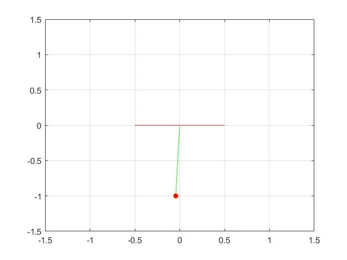
To animate the oscillation of a simple pendulum
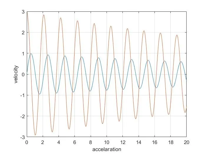
To plot displacement and velocity with respect to time.

Theory:

A simple pendulum consists of a large mass (bob) suspended by a light string from a rigid support. The length of the string is large compared to the dimensions of the bob. A stationary pendulum has its string in a vertical position with the bob hanging straight down. This is known as the pendulum's equilibrium position. Oscillations are set up in a pendulum by displacing the bob from its equilibrium position and releasing it.
In this simple pendulum, the oscillation comes to rest or equilibrium position after some time. this is because of the damping effect.
Damping is an influence within or upon an oscillatory system that has the effect of reducing, restricting, or preventing its oscillations. In a physical system, damping is produced by a process that dissipates the energy stored in the oscillation.
In addition to this, the same pendulum also describes the motion of the spring, mass, and damper system.

close all
clear all
clc

t = [0,20];
theta_0 = [0,3];

[t,theta] = ode45('simple_pendulum',t,theta_0);

plot(t, theta(:,1))
hold on
plot(t, theta(:,2))
grid on
xlabel('accelaration')
ylabel('velocity')

ct = 1;
for i = 1:length(theta(:,1))
    X = theta(:,1);
    X1 = X(i);
    x0 = 0;
    y0 = 0;
    l = 1;
    x1 = l*sin(X1);
    y1 = -l*cos(X1);
    %ploting pendulam
    figure(2)
    plot([-0.5 0.5],[0 0],'color','r');
    hold on
    plot([x0 x1],[y0 y1],'color','g');
    hold on
    plot(x1,y1,'marker','o','markerfacecolor','r');
    hold off
    grid on
    axis([-1.5 1.5 -1.5 1.5])
    M(ct) = getframe(gcf)
    ct = ct+1

end

movie(M)
videofile = VideoWriter('Forward_kinematics.avi','Uncompressed AVI')
open(videofile)
writeVideo(videofile,M)
close(videofile)

function[dtheta_dt] = simple_pendulum(t,theta,b,m,g,l)
dtheta_dt = zeros(2,1);
b = 0.05;
l = 1;
g = 9.81;
m= 1;
% theta = linspace(0,3,3)
dtheta_dt(1) = theta(2);
dtheta_dt(2) = (-b/m)*theta(2)-(g/l)*sin(theta(1));
end

https://youtu.be/ygiS84shaPI

https://drive.google.com/file/d/1PdcDh8s7r9wpsAwaQX2fD2cQSMOY3mn9/view?usp=sharing

RESULTS AND CONCLUSION:
1. Displacement and Velocity are calculated and plotted as shown above.
2. Animation of simulated 2nd order ODE is done and shown above.
3. Program is executed by breaking 2nd order ODE into 1st order ODE using MATLAB.