Week 3 - Solving second order ODEs

PROJECT REPORT

SOLVING SECOND ORDER ODEs USING PYTHON

AIM :

The objective is to write a program that solves the following ODE using odient solver. This ODE represents the equation of motion of a simple pendulum with damping.

THEORY :

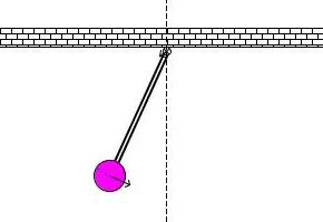
In Engineering, ODE is used to describe the transient behavior of a system. A simple example is a pendulum

The way the pendulum moves depends on the Newtons second law. When this law is written down, we get a second order Ordinary Differential Equation that describes the position of the "ball" w.r.t time.

This ODE represents the equation of motion of a simple pendulum with damping

In the above equation,

g = gravity in m/s2,

L = length of the pendulum in m,

m = mass of the ball in kg,

b = damping coefficient.

INPUT PARAMETRS :

L=1 m,

m=1 kg,

b=0.05.

g=9.81 m/s2.

Simulate the motion between 0-20 sec, for angular displacement=0,angular velocity=3 rad/sec at time t=0.

When you do this you will get the position of the pendulum as a function of time. Use this information to animate the motion of the pendulum, as shown in the below figure.

PYTHON CODE:

#Soving_second_order_odes

import math
from scipy.integrate import odient
import matplotlib.pyplot as plt
import numpy as np

#function that returns dz/dt
def model(theta,t,b,g,l,m):

    theta1 = theta[0]
    theta2 = theta[1]
    dtheta1_dt = theta2
    dtheta2_dt = -(b/m)*theta2 - (g/l)*math.sin(theta1)
    dtheta_dt = [dtheta1_dt, dtheta2_dt]
    return dtheta_dt

b = 0.05
g = 9.81
l = 1
m = 0.1

#initial condition
theta_0 = [0,3]

#time points
t = np.linspace(0,20,200)

#solve ODE
theta = odient(model,theta_0,t,args = (b,g,l,m))

#plot results
plt.plot(t,theta[:,0],'b-',label = r'$\frac{d\theta_1}{dt} = \theta2 $')
plt.plot(t,theta[:,0],'r--',label = r'$\frac{d\theta2}{dt} = \frac{b}{m}theta_2 - \frac{g}{l}sin\theta_1 $')
plt.xlabel('Time')
plt.ylabel('Plot')
plt.xlim([0, 12])
plt.legend(loc = 'best')
plt.show()

y = theta[:,0]
ct = 1
for angle in y:
    x1 = 0; y1 = 0;
    x2 = l*math.sin(angle)
    y2 = l*math.cos(angle)
    file = 'test%05d.png'%ct
    plt.figure()
    plt.plot([-0.5,0.5],[0,0],color='b',linewidth = 8)
    plt.plot([x1, x2],[y1, y2],color='r',linewidth = 3)
    plt.plot(x2,y2,'o',markersize = 15)
    plt.grid(color='b', ls = '-.', lw = 0.25)
    plt.xlim([-1.5, 1.5])
    plt.ylim([-1.5, 0.5])
    plt.savefig(file)
    ct = ct +1

RESULT :

1. PLOT OF DISPLACEMENT/VELOCITY vs TIME

2. Animation Video

YouTube Video Link : https://www.youtube.com/watch?v=P7mdDqTBHfs

ERROR :

Basic syntax errors are made during the first attempt of writing the programme later all of the errors are rectified.