Week 3 - Solving second order ODEs

Program : To solve a 2nd order ODE

close all
clear all
clc
% given condition
b = 0.05;
g = 9.81;
l = 1;
m = 1;

% initial condition
theta_0 =  [0,3];

% time points for 20 sec
t_span = linspace(0,20,500);

% solve ODE the function for ode_fun is already saved
% the function is 
% function [dtheta_dt] = ode_fun(t, theta, b, g, l, m)

% theta1 = theta(1)
% theta2 = theta(2)
% dtheta1_dt = theta2;
% dtheta2_dt = -(b/m)*theta2 - (g/l)*sin(theta1);
% dtheta_dt = [dtheta1_dt; dtheta2_dt];
% end

[t, results] = ode45(@(t,theta) ode_fun(t, theta,b,g,l,m), t_span, theta_0);
figure(1);
% the two results w.r.t are damping and 
plot(t,results(:,1));
hold on
plot(t,results(:,2));
ylabel('plot')
xlabel('time')

% Animation
ct = 1;
for i=1:length(t_span);
% cordinates of the pendulums are calculated
    x0 = 0; 
    y0 = 0;

    x1 = l*sin(results(i,1));
    y1 = -l*cos(results(i,1));
% for plotting the pendulum, ball and fix line in figure2 
    figure(2)
    plot([-1 1], [0 0],[x0 x1],[y0 y1],x1,y1,'o','markersize',20,'markerfacecolor','r');
    axis([-2 2 -2 2]);
    title('Simple Pendulum');
    legend('Support rod','length of pendulum','Mass of ball');
    grid on
    pause(0.03) % pause for 0.03 sec to have smooth animation 
    % getting all the individual frames in an arry called M
        % using getframe command to get current figure window
    M(ct) = getframe(gcf);
       % first svae the frame and then increment the counter
    ct = ct + 1;
end
% to genreate a move using all the frame movie(m) command is used    
movie(M)
% creating a video file by using videoWriter
videofile = VideoWriter('simple_pendulum.avi','Uncompressed AVI');
% the video file will be open and then it will be played and closed
open(videofile)
writeVideo(videofile,M)
close(videofile)

Explanation :

Step1 : The first step is to solve the ODE by assuming theata = theata1, dtheata1/dt = theata2 that will solve the ODE in the form of theata1 and theata2 which in matrix forma is written.

Step2 : After Solving represting it in the programing language

Step3 : Considering all the given value and mentioning and representing them,

Step4 : Then Defining the initial condition of the pendulum

Step5 : Now solving the ODE with matlab function ode45(@(t,theta) ode_fun(t, theata, b, g, l, m),t_span,theta_0). here the ode_fun is function made to solve the equation of the of 2nd order differential. where we get the two results for velocity and damping.

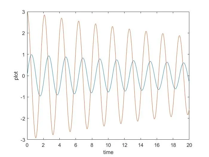
Step6 : The ploting of the graph is done using figure(1) command, where ploting of two graph is don in same fig with hol on command.

Step7 : Now ploting the pendulum in figure(2), where the support rod, length of the pendulum, and the mass of the ball is ploted with single command,

Step7 : Then the animation is done using the for loop, counter and movie command.

Step8 : hence the animation is generated and graph also gets ploted which completes the program.

Graph : Damping and Velocity with respect to time

Youtube Link : Simple Pendulum Animation

Simple pendulum

Error :

1) The equation defining in the function also had many confusing but after repeatative watching of video gave an idea to write the equation in programing language.

2) The ploting of pendulum was not comming as the angle needed to be define in the for loop command so which results to take was bit confusing and then results(i,1) was finally understood to take.