Week 3 - Solving second order ODEs

kindly click on the link for the animation of the pendulum.

https://drive.google.com/file/d/1vA8xnXGD7t8rAp5DudcRzKMkjiUgIOxF/view?usp=sharing

1. AIM: Simulate the motion of the pendulum

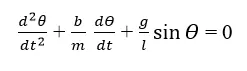
2. GOVERNING EQUATIONS:

use the following parameters in the given equation'

g = 9.81 [gravity in m/s2],

l = 1 [length of the pendulum in m],

m = [1 mass of the ball in kg],

b=0.05 [damping coefficient].

3. OBJECTIVE:

Use the following equation to solve the second order differential equation for the simple pendulum in damping.

4. BODY OF THE CONTENT:

• The function is first created and the main program is written.
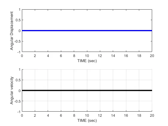
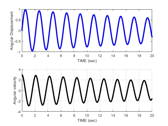
• The first subplot is created for angular displacement wrt to time.
• The second subplot is created for angular velocity wrt to time.
• function is written for the animation in the main program.
• we have assumed the null matrix to xdot.
• in the function x is using instead of theta and xdot is output variable for the function.
• the xdot(2) in the function will obtain after conversion of secon order ODE to first order.
• animation link is provided.

  function xdot=pendulum_second_order(t,x) %use x instead theta
  b=0.05;
  g=9.81;
  l=1;
  m=1;
  xdot=zeros(2,1);
  % first element is angular velocity at x(2) position
  xdot(1)=x(2);
  xdot(2)=-(b/m)*x(2)-(g/l)*sin(x(1));
  
  end
  
  ​
  clear all
  close all
  clc
  
  l=1;
  t=linspace(0,20,500);
  x0=[0 3];
  [t x]=ode45('pendulum_second_order',t,x0);
  
  
  subplot(2,1,1)
  plot(t,x(:,1),'-b','LineWidth',3);
  xlabel('TIME (sec)');
  ylabel('Angular Displacement');
  
  subplot(2,1,2)
  hold on;
  plot(t,x(:,2),'-k','LineWidth',3);
  xlabel('TIME (sec)');
  ylabel('Angular velocity');
  grid on;
  
  
  %animation
  X0=0;
  Y0=0;
  ct=1;
  
  for i=1:length(t)
      X1=l*sin(x(i,1));
      Y1=-l*cos(x(i,1));
  
      figure(2)
      plot([-1 1],[0 0],'lineWidth',6,'Color','g');
      axis([-2 2 -2 2]);
      line([X0 X1],[Y0 Y1],'linewidth',6,'color','b');
      hold on;
  
      plot(X0,Y0,'O','MarkerSize',3,'MarkerFaceColor','y');
      plot(X1,Y1,'O','MarkerSize',15,'MarkerFaceColor','r');
      title('Damping of pendulum');
      legend('support rod','length of pendulum','fixed point','pendulum bob');
      grid on;
      hold off;
      M(ct)=getframe(gcf);
      ct=ct+1;
  
  end
  
  movie(M);
  videofile=VideoWriter('pendulum','MPEG-4');
  open(videofile);
  writeVideo(videofile,M);
  clode(videofile);
  
  
  
  
  
         
  
  
  
    
  
  
  
  
  
  

5. CONCLUSION:

• The plot is generated showing the angular displacement and angular velocity wrt time
• the mass of the bob is 1 kg, and the plot is generated with angular displacement 0 and angular velocity 3 rad/sec at time t=0 sec.
• the animation is created. click on the link at start.
•