Week 3 - Solving second order ODEs

AIM :

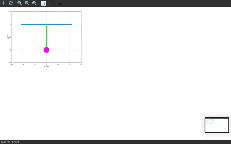
Your objective is to write a program that solves the following ODE. This ODE represents the equation of motion of a simple pendulum with damping Simulate the motion between 0-20 sec, for angular displacement=0,angular velocity=3 rad/sec at time t the position of the pendulum as a function of time. Use this information to animate the motion of the pendulum, as shown in the figure.

FOLLOWING PARAMETERS :

GRAVITY g=9.81 m/s2

LENGTH OF THE PENDULUM l=1m,

MASS OF THE BALL m=1 kg,

DAMPING CO-EFFICIENT b=0.05.

TIME t =[0-20]sec

ANGULAR DISPLACEMENT = 0

ANGULAR VELOCITY = 3 RAD/SEC^2(AT t =0)

GIVEN EQUATION :

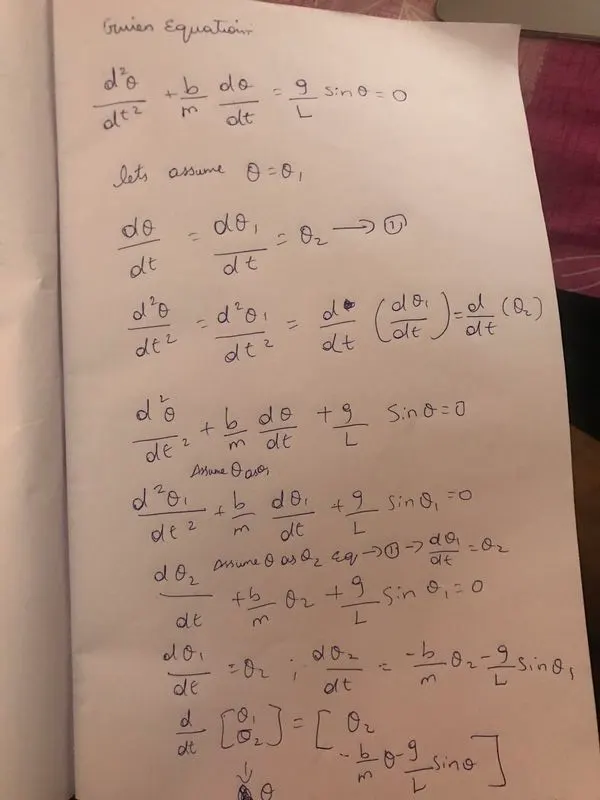
lets sey :

θ = θ1

(d(θ)/dt)=θ2

(d^2θ/dt)=( d^2θ1/dt^2) =d/dt d(θ)/dt=d/dt(θ2)

programs in octave and matlab

main code :

clear all
close all 
clc

b=0.05;
g=9.81;
l=1;
m=1;

%we need to represent initial condition 
theta_0=[0;3];

%given time intervals
t_span = linspace(0,20,400);

%solve ODE
[t,results] = ode45(@(t,theta)ode_func(t,theta,b,g,l,m),t_span,theta_0);

figure (1)
plot(t,results(:,1))
hold on 
plot(t,results(:,2))
xlabel('time')
ylabel('Angular displacement vs Angular velocity')
legend('Angular displacement','Angular velocity')
grid on
figure (2)
plot(results(:,1),results(:,2))
xlabel('postion')
ylabel('Angular velocity')
legend('Angular velocity')

theta2=results(:,1)
ct =1
for i =1:length(theta2)
  theta3 =theta2(i)
  % for fixed bar and moving bar of the pendulum
  x0=0
  y0=0
  x1 = 1*sin(theta3)
  y1 = -1*cos(theta3)
  % giving axis , color for pendulum bob , 
  figure (3)
  plot([-1.1 1.1],[0,0],'linewidth',3)
  hold on
  plot([x0 x1],[y0 y1],'g','linewidth',3)
  hold on
  plot(x1,y1,'o','markers',20,'markerfacecolor','M')
  xlabel('x-axis')
  ylabel('y_axis')
  hold off
  grid on 
  axis([-1.5 1.5 -1.5 0.5])
  % time frame to get the video 
  pause (0.003)
  M(ct) = getframe(gcf)
  ct + ct+1
  end
  % code to run and save the video 
  movie(M)
  videofile = videowriter ('simple pendulum.avi','uncompressed AVI')
  open (videofile)
  writevideo(videofile,M)
  close (videofile)
  

function code :

function[dtheta_dt]= ode_func(t,theta,b,g,l,m)
theta1 = theta(1)
theta2 = theta(2)
dtheta1_dt= theta2;
dtheta2_dt= -(b/m)*theta2 - (g/l)*sin(theta1);
dtheta_dt= [dtheta1_dt; dtheta2_dt];
end

RESULT:

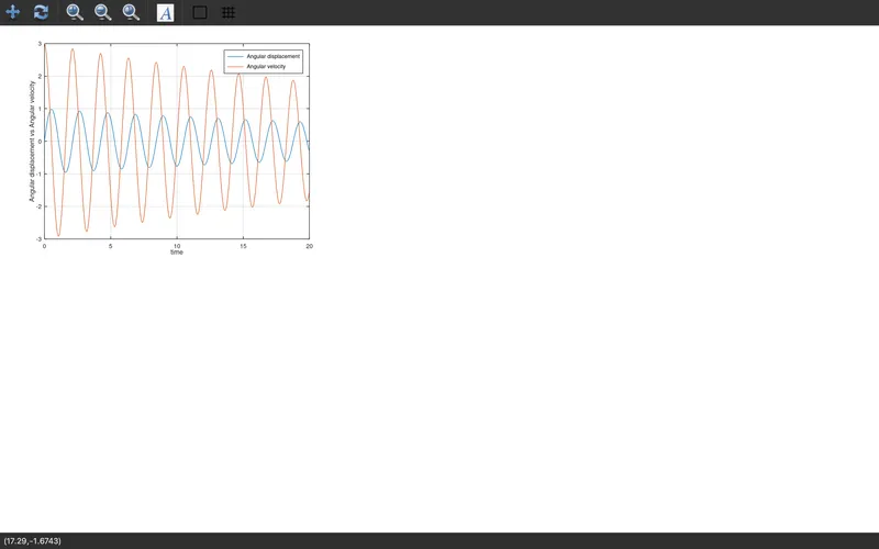
TIME VS ANGULAR DISPLACEMENT AND ANGULAR VELOCITY :

The plot explains how the angular velocity and angular displacement is varying with respect to time

we can observe here how angular velocity and displacement are changing with respect to time

POSITION VS ANGULAR VELOCITY :

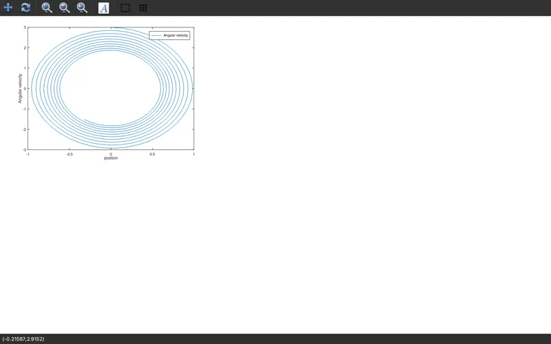
plot explains to us the position of bob or ball on the scale of [-11] while its angular velocity is going to decrease gradually

the bob in the simple pendulum starts at a point at a velocity of 3m/s and as the solution starts the bob slowly lost its momentum and made the impression of the path

after the given times of 20 sec the velocity reaches nearly 1.3m/s

PENDULUM: