Week 3 - Solving second order ODEs

Solving second order ODEs – Challenge

Here, is the animation of the pendulum derived from calculating the mentioned ODE problem-

https://drive.google.com/file/d/18MQMlnz9YeZCh9NQbGD5c8LX2tYrMG6G/view?usp=sharing

Here, is the code used to get the create the animation of the pendulum-

clear all
close all
clc


b = 0.05;
g = 9.81;
l = 1;
m = 1;


% Initial Condition
theta_0 = [0;3];

% Time points
t_span = linspace(0,20,480);

% solve ODE
[t, results] = ode45(@(t, theta)second_order_ODEs_func_challenge (t, theta, b, g, l, m), t_span, theta_0);

% Now, for creating a Pendulum Animation

% To plot a line with length and angle

normal_position = 270*pi/180;
displacement_theta = results(:,1);
f_theta = normal_position + displacement_theta;

% Pause time for the animation
pt = 0.04;

% Fixed point of the string
x0 = 0;
y0 = 0;

% Loop Counter
ct = 1;

  for i = 1:length(t_span)
  
  x1 = (l * cos (f_theta(i))) + x0;
  y1 = (l * sin (f_theta(i))) + y0;
  
  
  plot ([x0],[y0],'*',[x1],[y1],'-o','Markersize',20,[x0 x1],[y0 y1]);
  axis([-1.5 1.5 -2 0.5]);
  grid on;
  xlabel ('X-axis');
  ylabel ('Y-axis');
  title ('Representation of the moving pendulum');
  
  % Animation Commands
  pause(pt);
  printf ('Creating GIF - Progress.... %d/%dn', ct, length (displacement_theta));
  img = print ('-RGBImage');
  imwrite (img, 'Animation.gif', 'DelayTime', pt, 'Compression', 'bzip', 'WriteMode', 'Append');
  
  ct = ct+1;

endfor

& here, is the code of the function called in the above code,

function [dtheta_dt] = second_order_ODEs_func_challenge(t, theta, b, g, l, m)


  theta1 = theta(1);
  theta2 = theta(2);
  dtheta1_dt = theta2;
  dtheta2_dt = -(b/m)*theta2 - (g/l)*sin(theta1);
  dtheta_dt = [ dtheta1_dt; dtheta2_dt];
  
  endfunction

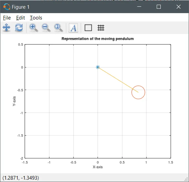
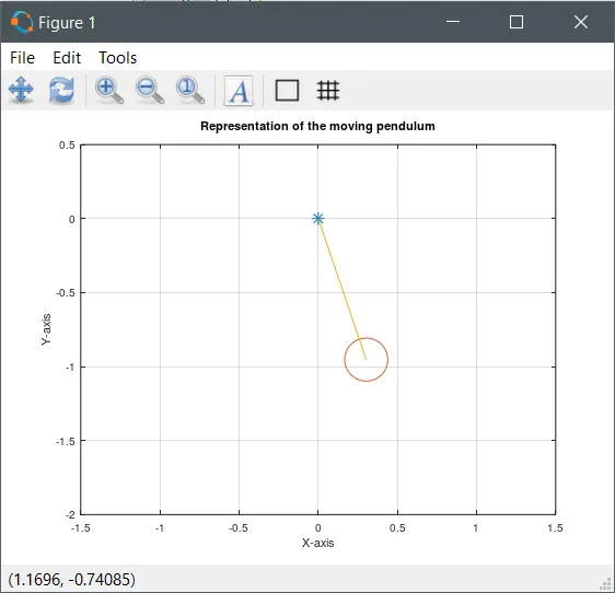
& here, is the output screen shot of the code-

Now, as for the explanation of the code used to solve the said ODE,

clear all
close all
clc


b = 0.05;
g = 9.81;
l = 1;
m = 1;


% Initial Condition
theta_0 = [0;3];

% Time points
t_span = linspace(0,20,480);

Here, I just initiated all the parameters that’ll be used in the code for solving the ODE equation, where, g = gravity - 9.81 m/s2.,
L = length of the pendulum - 1m.,
m = mass of the ball – 1 kg.,
b = damping coefficient – 0.05.

And the initial conditions of the angular displacement & angular velocity at time = 0, are placed in ‘theta’ variable array as 2 elements in different columns.

And the time span is taken from 0 to 20 secs, as mentioned in the question, & is initiated as ‘t_span’ variable using linspace.

% solve ODE
[t, results] = ode45(@(t, theta)second_order_ODEs_func_challenge (t, theta, b, g, l, m), t_span, theta_0);

Here, to solve the ODE equation, calling a function i.e., ‘ode45’ function, as it is a inbuilt function used to solve ODE equations, the syntax is as follows-

[t,results] – the results after solving the ODE are put in a ‘results’ array,

ode45(@(t, theta) - this is the syntax for calling the ode45 solver with the variables it is supposed to solve for in the function called right after it,

second_order_ODEs_func_challenge (t, theta, b, g, l, m) - this is the syntax for calling the function where the ode45 solver is to be used with its output variables as ‘t,theta’ & other input arguments ‘b, g, l, m’ etc.

Here, the function ‘second_order_ODEs_func_challenge’, is a separate function / program used to convert and simplify the second order ODEs into first order ODEs, explanation for that code will be explained later in the report.

& t_span, theta_0) - the last part of calling the ode45 solver, the time span or the solving limits and the initial conditions for the problem are specified here.

% Now, for creating a Pendulum Animation

% To plot a line with length and angle

normal_position = 270*pi/180;
displacement_theta = results(:,1);
f_theta = normal_position + displacement_theta;

% Pause time for the animation
pt = 0.04;

% Fixed point of the string
x0 = 0;
y0 = 0;

% Loop Counter
ct = 1;

  for i = 1:length(t_span)
  
  x1 = (l * cos (f_theta(i))) + x0;
  y1 = (l * sin (f_theta(i))) + y0;
  
  
  plot ([x0],[y0],'*',[x1],[y1],'-o','Markersize',20,[x0 x1],[y0 y1]);
  axis([-1.5 1.5 -2 0.5]);
  grid on;
  xlabel ('X-axis');
  ylabel ('Y-axis');
  title ('Representation of the moving pendulum');
  
  % Animation Commands
  pause(pt);
  printf ('Creating GIF - Progress.... %d/%dn', ct, length (displacement_theta));
  img = print ('-RGBImage');
  imwrite (img, 'Animation.gif', 'DelayTime', pt, 'Compression', 'bzip', 'WriteMode', 'Append');
  
  ct = ct+1;

endfor

Now, this last segment of the code is only for plotting and animating the results obtained from solving the ODE equation in the previous section,

Here,
normal_position = 270*pi/180, is the angle of the string when it is at rest, that is at 270 degrees, converted to radians, as the angular velocity given in the question was in radian/seconds.

displacement_theta = results(:,1), here, I’ve separated the angular displacement results from the ‘results’ variable, and placed it in the ‘displacement_theta’ variable for further simpler use,

f_theta = normal_position + displacement_theta, here, I’ve made a statement that will let me calculate the final position of the string w.r.t. to the normal position using the displacement_theta’ variable.

After that I’ve initiated pause time for the animation, the fixed position of the string as (0,0) and a loop counter variable.

After that, initiating a ‘for’ loop, where for each value of time,
end position of the pendulum is calculated using the formula for the coordinates x1 & y1 as mentioned in the code,
and plotted with ‘marker’ property as well, so as to represent a spherical mass.

Then, we, use the animation commands, where the ‘pause’ command is used to pause the plot result for the specified value of ‘pt’ variable before showing the next result;

the ‘pause’ command used here does not govern the pausing time for the animation file, it just pauses the output,

The ‘printf’ command used here, helps in keeping track of the GIF creation process,

Then, the ‘print’ command is used to fetch the current plot image & store it in the ‘img’ variable,

Then, the command ‘imwrite’ is used to write images or plots into various specified formats,

here, ‘img’ is the variable where the plot is stored,

& ‘Animation.gif’ is the name & format of the file,

& ‘DelayTime’ is the property used to specify the delay time between frames for the GIF file,

& ‘Compression’ is the property used to compress the image files so that they can be compressed to the minimum size possible for GIF creation,

& ‘WriteMode’ is the property used for specifying the writing mode of the frames in the animation gif, which here is ‘Append’.

Lastly, increment for the loop counter ‘ct’, and 'endfor' command to mark the end point for both the ‘for’ loops.

Now, all of this code will be executed again & again for all the values of time i.e. ‘t_span’ due to the condition of the 'for' loops,

and each time they are executed, a new plot frame is added to the GIF file which is being created.

Here, is the explanation for the function called for the ode45 solver –

function [dtheta_dt] = second_order_ODEs_func_challenge(t, theta, b, g, l, m)


  theta1 = theta(1);
  theta2 = theta(2);
  dtheta1_dt = theta2;
  dtheta2_dt = -(b/m)*theta2 - (g/l)*sin(theta1);
  dtheta_dt = [ dtheta1_dt; dtheta2_dt];
  
  endfunction

Here, the equation governing the motion of the pendulum is as such,

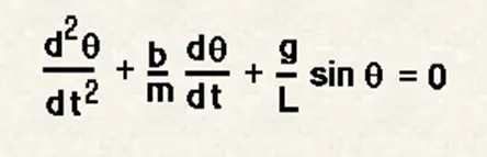
where,

g = gravity in m/s2,
L = length of the pendulum in m,
m = mass of the ball in kg,
b = damping coefficient.

And θ here, is the angular displacement in radians, and t is time in seconds.

The ‘function’ command at the start lets us use this program in other programs whenever needed by function calling.

The ‘second_order_ODEs_func_challenge’ is the name of the program, & (t, theta, b, g, l, m) are the inputs needed to call & execute the function wherever we need.

Then, initial condition angular displacement element theta(1) is assigned to variable ‘theta1’, and similarly, initial condition angular velocity element theta(2) is assigned to variable ‘theta2’.

Substituting,
dθ₁ / dt = theta2,
and subsequently, dθ₂ / dt = -(b/m)*theta2 - (g/l)*sin(theta1).

Above is the simplification of second order ODE into first order ODE.

Lastly, ‘endfunction’ command is used to denote the end of the code under the ‘function’ command.

Errors faced while Programming –

Error -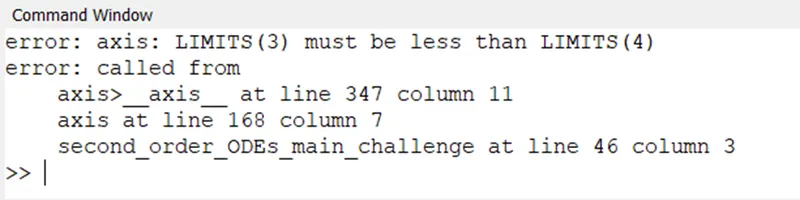

As per the above error, the axis command has to have the Y axis limits which is the 3^rd limit & the 4^th limit values, there the 3^rd limit should be less than the 4^th limit,

Earlier it was as such,

, then rectified it to

That solved the error.

Error -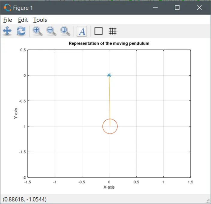

The output pendulum was not moving much, this didn’t show as an error but such output was not much help to be presented,
after close inspection of the question and the code, I found out that the velocity in the question is given as 2 rad/s, which means that the angular displacement is also in radians, and the formula that I’ve used for calculating x1 & y1 coordinates for the end point of the pendulum should have ‘cos’ & ‘sin’ commands instead of ‘cosd’ & ‘sind’, which are used for displacement in degrees,

So rectified the code from,

To,

and also rectified the normal_position to radians as such,


That, solved the error and gave proper plots.