Week 3 - Solving second order ODEs
Aim : Solving second Order ODEs
objective :
to write a program that solves the ODE. represents the equation of motion of a simple pendulum with damping
Given data :
L=1 metre,
m=1 kg,
b=0.05.
g=9.81 m/s2.
note:
g = gravity in m/s2,
L = length of the pendulum in m,
m = mass of the ball in kg,
b=damping coefficient.
Simulate the motion between 0-20 sec,
for angular displacement=0,
angular velocity=3 rad/sec at time t=0.
solution :
To solve 2nd order ODEs we have to brake down equation into first oder and hence the the equation will be as follows
Assume that
[d(theta1)] /[d(time)] = theta2
hence by solving pendulum equation will get following equation
[d(theta2)]/[d()time] = -(b/m)*theta2 - (g/l)*sin(theta1)
hence will write the program as bellow
% function code

function xdot = pendulum_2nd_order(t,theta)
% Inputs
b = 0.05
g = 9.81;
l = 1;
m = 1;

xdot = zeros(2,1)
xdot(1) = theta(2)
xdot(2)  = -(b/m)*theta(2) - (g/l)*sin(theta(1));
end
first give the input for function and then specify the renge for the working parameter
xdot will be the output variable for function
and also the provide the woking formula for the function
give the file name same as function name so when we call the function it will work properly for the program.
Program script :
starting with
clear all
close all
clc
for the previous work should be clear and it should not mix with latest results
hence the maim thing is to first give input and interval for time (0,20)
in matlab special function ode45:
which work on variable step Runge-Kutta Method to solve differential equations numerically
ODE45 is usually the function of choice among the ODE solvers. It compares methods of orders four and five to estimate error and determine step size
% For the second order degree solving
clear all
close all
clc

l = 1;
t = linspace(0,20,150);
theta0 = [0 3];

% solve ODE
[t theta] = ode45('pendulum_2nd_order', t,theta0);

%ploting for the tracing of angulur velocity and angular displacement
subplot(2, 1, 1)
plot(t, theta(:,1),'-b','linewidth',3);
xlabel('time t in sec');
ylabel('Angulular displacement');
subplot(2,1,2)
hold on

plot(t, theta(:,2),'-k','linewidth',3)
xlabel('time t in sec');
ylabel('Angulular velocity');
grid on
hence trace the plot which shows the velocity vs dispalcement with respect to angle
hence with this program result will be as follow
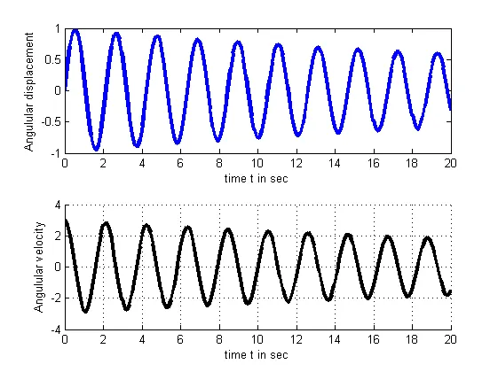
hence for the animation of the of the pendulum rotation program should be continued as follows
take the position from origin of (0,0) of x, y coordinates
ct= counter represents each and every frame
ct = 1
here the main use of for loop :
A for loop is a repetition control structure that allows the program efficiently work a loop that needs to execute a specific number of times. The syntax of a for loop in MATLAB is as following
for i = 1:length
provide the structure for pendulum as bellow
markersize
markerfacecolor
Support rod
Length of pendulum
Fixed points
Bod of pendulum
hance create movie folder for animation save
%Animation
x0 = 0;
y0 = 0;

% ct counter represents each and every frame
ct = 1;
for i = 1:length(t)

x1 = l*sin(theta(i,1));
y1 = -l*cos(theta(i,1));

  figure(2)
plot([-1 1],[0 0],'linewidth',6,'color','g');
axis([-2 2 -2 2]);
line([x0 x1],[y0 y1],'linewidth',2, 'color','b');
hold on ;
plot(x0, y0, 'o', 'markersize',3, 'markerfacecolor', 'y');
plot(x1, y1, 'o', 'markersize',20, 'markerfacecolor', 'r');
title('Damping of simple pendulum');
legend('Support rod','Length of pendulum','Fixed points','Bod of pendulum');
grid on ;
hold off;
M(ct)=getframe(gcf);
ct=ct+1;
end

movie(M);
videofile = VideoWriter('simple_pendulum','Uncompressed AVI');
open(videofile);
writeVideo(videofile,M);
close(videofile);
and complete program will be as bellow
% For the second order degree solving
clear all
close all
clc

l = 1;
t = linspace(0,20,150);
theta0 = [0 3];

% solve ODE
[t theta] = ode45('pendulum_2nd_order', t,theta0);

%ploting for the tracing of angulur velocity and angular displacement
subplot(2, 1, 1)
plot(t, theta(:,1),'-b','linewidth',3);
xlabel('time t in sec');
ylabel('Angulular displacement');
subplot(2,1,2)
hold on

plot(t, theta(:,2),'-k','linewidth',3)
xlabel('time t in sec');
ylabel('Angulular velocity');
grid on

%%
%Animation
x0 = 0;
y0 = 0;

% ct counter represents each and every frame
ct = 1;
for i = 1:length(t)

x1 = l*sin(theta(i,1));
y1 = -l*cos(theta(i,1));

  figure(2)
plot([-1 1],[0 0],'linewidth',6,'color','g');
axis([-2 2 -2 2]);
line([x0 x1],[y0 y1],'linewidth',2, 'color','b');
hold on ;
plot(x0, y0, 'o', 'markersize',3, 'markerfacecolor', 'y');
plot(x1, y1, 'o', 'markersize',20, 'markerfacecolor', 'r');
title('Damping of simple pendulum');
legend('Support rod','Length of pendulum','Fixed points','Bod of pendulum');
grid on ;
hold off;
M(ct)=getframe(gcf);
ct=ct+1;
end

movie(M);
videofile = VideoWriter('simple_pendulum','Uncompressed AVI');
open(videofile);
writeVideo(videofile,M);
close(videofile);
- Errors while solving the ODEs:
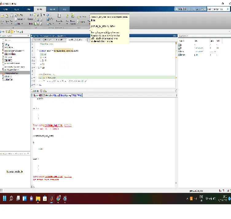
here you have to put same file name as function without giving gap in it. it will also show the not enough aurguments, hence you will overcome this
- animation video will be as : (link is provided as bellow):
with this attachment the solution is provided as
- Plot for the velocity vs displacement.
- pendulum function program .
- code for the program.