Week 3 - Solving second order ODEs
Simulation of the Motion of a Simple Pendulum using Matlab
Objective:
- To simulate the motion of a simple pendulum
- To create an animation of its motion
Theory:
A simple pendulum consists of a mass m hanging from a string of length L and fixed at a pivot point P. When displaced to an initial angle and released, the pendulum will swing back and forth with periodic motion. By applying Newton's secont law for rotational systems, the equation of motion for the pendulum may be obtained as follows:
`\frac{d^{2}\theta}{dt^2} + \frac{g}{L} sin(\theta) = 0`
However, there exist the presence of air resistance which slows down the motion of a simple pendulum and acts as a damping factor. As a result of the presence of resisting force, the velocity of the mass decreases. This is called a damped simple harmonic motion.
From Newton's Second Law of Motion, a second order ordinary differential equation (ODE) defines the relationship of the angular displacement with time is given as:
`\frac{d \theta_1}{dt} - \theta_{2} = 0`
`\frac{d^{2}\theta}{dt^2} + \frac{b}{m} \frac{d\theta}{dt} + \frac{g}{L} sin(\theta) = 0`
The terms of the equation above are θ = angular displacement in radians, g = acceleration due to gravity in m/s^2, L = length of the pendulum in m, m = mass of the ball in kg, and b=damping coefficient.
MATLAB Code:
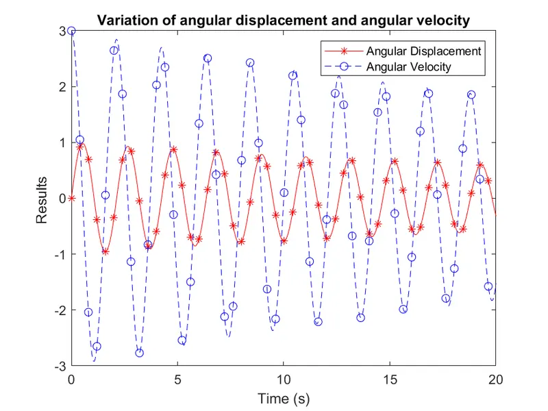
Simulation of the motion of a simple pendulum is a way of visualizing the variation of angular displacement () and angular velocity ( ) wrt time. A second order Ordinary Differential Equation (ODE) given above is integrated numerically within the given time interval using a Matlab function ode45 which solves a first order differential equation. However, the governing equation of a simple pendulum is a 2nd order ODE. To surmount this limitation, the 2nd order ODE is transformed into a linear system of first order ODEs which are given as:
`\frac{d\theta_{2}}{dt} + \frac{b}{m} \theta_{2} + \frac{g}{L} sin(\theta_{1} ) = 0`
%Input Parameters:
clear all
clc
close all

% Input parameters for simulation of the motion of asimple pendulum
sprintf('Inputs for simulation of the motion of a simple pendulum :')

% Mass of the ball (kg)
mass = 1;
sprintf('Mass of the ball (kg), m = %0.4f', mass)

%Length of the pendulum (meter)
pend_length = 1;
sprintf('Length of the pendulum (meter), L = %0.4f', pend_length)


% Damping Coefficient
damp_coeff = 0.05;
sprintf('Damping Coefficient, b = %0.4f', damp_coeff)

% Acceleration due to gravity (m/s^2)
acc_gravity = 9.81;
sprintf('Acceleration due to gravity (m/s^2), g = %0.4f', acc_gravity)


% Initial Conditions i.e value of angular displacement i.e theta = 0 and angular velocity i.e omega = 3 rad/s at t = 0
initial_angle = [0; 3];
sprintf('Initial Conditions, y0 = %0.4f', initial_angle)

% Defining time interval required for simulation of simple pendulum (second)
t_interval = linspace(0, 20, 500);
sprintf('Time Interval, t_span = %0.4f', t_interval)


% Define the system of ODE
ode_func = @(t, theta) [theta(2); -acc_gravity/pend_length * sin(theta(1)) - damp_coeff ./ mass .* theta(2)];

% Solve the System of ODE:
% Solving a system of first order differential equation using
% Result Array
[time, solution] = ode45(ode_func, t_interval, initial_angle);

% Plot the Variation of angular displacement and angular velocity with time

% Plotting the variation of angular displacement and angular velocity with respect to time
fig = figure();
plot(t_interval, solution(:,1),'-*',"Color", 'r','MarkerIndices',1:10:length(t_interval))
ax = gca;
ax.NextPlot = 'add';
plot(t_interval, solution(:,2),'--o',"Color", 'b','MarkerIndices',1:10:length(t_interval))

% Add title, axis label, and legend to the plot
title("Variation of angular displacement and angular velocity")
xlabel("Time (s)")
ylabel("Results ")
legend({'Angular Displacement', 'Angular Velocity'})

saveas(fig,'Variation_angular_displacement_velocity.png')

% Animation:
% Create an animation of the simple pendulum
% Compute the location of the pendulum
% The Origin
X0 = 0;
Y0 = 0;
X = pend_length * sin(solution(:,1));
Y = -pend_length * cos(solution(:,1));

% Creat an animation
% Create a figure for the animation
fig1 = figure();

% Plot for creating support
%plot([-1, 1], [0, 0], color = 'r', linewidth = 3)
ax = gca;
ax.NextPlot = 'replace';

ct = 1;
Mov = struct('cdata',[], 'colormap', []);
for intJ = 1 : length(time)

    % Plot for creating support
    plot([-1, 1], [0, 0], color = 'r', linewidth = 3)
    hold on;
    % Plot for creating the pendulum string
	plot([X0, X(intJ)], [Y0, Y(intJ)], color = 'k', linewidth = 3)

	% Plot for creating a ball of the pendulum
	plot(X(intJ), Y(intJ), marker = 'o', markerfacecolor = 'm', markeredgecolor = 'k', markersize = 20)

	% Inserting the text in a plot
    xtext = ['Angular Displacement = ' ,  num2str(solution(intJ,1)) , ' rad'];
    angText = ['Angular Velocity = ' , num2str(solution(intJ, 2)) , ' rad/s'];
	text(-1, 0.3, xtext, color = 'c')
	text(-1, 0.1, angText, color = 'm')
    title("Motion of a Simple Pendulum")
    xlabel("Horizontal Displacment [m]")
    ylabel("Vertical Displacement [m]")
    axis([-1.5, 1.5, -1.5, 0.5])
    pause(0.1)
    hold off;
    Mov(ct) = getframe(gcf);
    ct = ct + 1;

end

% Write the movie frames to a video file.
movie(Mov)
videofile = VideoWriter('Simple_pendulum.avi','Uncompressed AVI');
open(videofile)
writeVideo(videofile, Mov)
close(videofile)
Output:
Explanation of Code :
Defining inputs and and getting them print:
- Mass of ball of the pendulum (kg) - mass = 1
- Length of the string of the pendulum (meter) - pend_length = 1
- Damping coefficient - damp_coeff = 0.05
- Acceleration due to gravity (m/s^2) - acc_gravity = 9.81
- Array with first element of row as angular displacement (rad) and second element of row as angular velocity (rad/s) - initial_angle = [0; 3]
- Time interval of 20 seconds divided into 500 parts and presented as a row vector - t_interval = linspace(0, 20, 500)
System of ODE:
A function ode_func is defined to compute the system of ODE. This is defined as inline function as
- ode_func = @(t, theta) [theta(2); -acc_gravity/pend_length * sin(theta(1)) - damp_coeff ./ mass .* theta(2)];
This function handler will be used to solve the ODE using the matlab function ode45 as shown below.
Solve the System of ODE
The system of ODE is solved with the code:
- [time, solution] = ode45(ode_func, t_interval, initial_angle);
such that time is time of the computed angular displacement and angular velocity of the simple pendulum stored in the variable solution. The ode45 is a matlab ode solver which uses the defined system of ODE ode_func, the time interval t_interval, and the initital condition initial_angle to solve the system of ODEs.
Plot the variation of angular displacement and angular velocity as function of time:
The plot of the variation of angular displacement and angular velocity are generated by creating a figure pallete which will hold the plots generated using the code: fig = figure(). The axes of the figure are assigned to ax then the plots of angular displacement and angular velocity are plotted on the generated figure fig with this code snippets:
- % Plotting the variation of angular displacement and angular velocity with respect to time
fig = figure();
plot(t_interval, solution(:,1),'-*',"Color", 'r','MarkerIndices',1:10:length(t_interval))
ax = gca;
ax.NextPlot = 'add';
plot(t_interval, solution(:,2),'--o',"Color", 'b','MarkerIndices',1:10:length(t_interval)) - % Add title, axis label, and legend to the plot
title("Variation of angular displacement and angular velocity")
xlabel("Time (s)")
ylabel("Results ")
legend({'Angular Displacement', 'Angular Velocity'})
The title, axes label and the legends of the plot created are added to the plots as shown in figures above.
Creation of the Animation of the motion of the Simple Pendulum.
To animate the motion of the simple pendulum, the location of the mass (X,Y) at each is computed using the following code:
- % Compute the location of the pendulum
% The Origin
X0 = 0;
Y0 = 0;
X = pend_length * sin(solution(:,1));
Y = -pend_length * cos(solution(:,1)); - At each time in space, the location of the mass and string is plotted and captured into a videoframe using the code below:
% Creat an animation
% Create a figure for the animation
fig1 = figure(); - % Plot for creating support
%plot([-1, 1], [0, 0], color = 'r', linewidth = 3)
ax = gca;
ax.NextPlot = 'replace'; - ct = 1;
Mov = struct('cdata',[], 'colormap', []);
for intJ = 1 : length(time)
% Plot for creating support
plot([-1, 1], [0, 0], color = 'r', linewidth = 3)
hold on;
% Plot for creating the pendulum string
plot([X0, X(intJ)], [Y0, Y(intJ)], color = 'k', linewidth = 2) - % Plot for creating a ball of the pendulum
plot(X(intJ), Y(intJ), marker = 'o', markerfacecolor = 'm', markeredgecolor = 'k', markersize = 15) - % Inserting the text in a plot
xtext = ['Angular Displacement = ' , num2str(solution(intJ,1)) , ' rad'];
angText = ['Angular Velocity = ' , num2str(solution(intJ, 2)) , ' rad/s'];
text(-1, 0.5, xtext, color = 'r')
text(-1, 0.2, angText, color = 'b')
axis([-1.5, 1.5, -1.5, 1])
pause(0.1)
hold off;
Mov(ct) = getframe(gcf);
ct = ct + 1;
end - % Write the movie frames to a video file.
movie(Mov)
videofile = VideoWriter('Simple_pendulum.avi','Uncompressed AVI');
open(videofile)
writeVideo(videofile, Mov)
close(videofile)
In this code, the video frame is captured from the generated plot at each time of the motion and added to the movie variable Mov. After capturing all the video frames of the motion, the video frame is converted into a video and written to a video file. The generated video is attached to the youtube link as shown below.
There was no issue with generating the code.