Week 3 - Solving second order ODEs

The following code was written to simulate the oscillation motion of a pendulum using second-order ODEs:

close all
clear all
clc

b = 0.05;
g = 9.81;
l = 1;
m = 0.1;
%initial conditions
ang_v = 3;
theta_0 = [0;3];
t_span = linspace(0,20,500);
ct=1
for i = 1:length(t_span)
% time points

    %solve ode
[t, results] = ode45(@(t,theta) ode_func(t, theta, b,g,l,m),t_span, theta_0);

%defining line of pendulum
x1 = 0;
y1 = 0;
x2 = -l*sin(results(i,1));
y2 = -l*cos(results(i,1));
plot([x1 x2], [y1,y2],'-or','linewidth',4)
axis ([-0.8 0.8 -1.2 0.4])

pause(0.01)
M(ct) = getframe(gcf);
ct = ct+1;
end
% Making a Video file
        movie(M)
        videofile = VideoWriter('pendulam.avi','Uncompressed AVI')
        open(videofile)
        writeVideo(videofile,M)
        close(videofile)

The link to the output video file of the above code is as follows: https://youtu.be/C3_7Cv9lI6E

The explanation for the code is as follows:

• The code has first started with the standard commands close all, clear all and clc to clear the workspace and command Window
• Then the values of the inputs b,g,l,m were assigned
• Then the initial condition for the pendulum was defined
• Then a for loop was used, running for each value of the timespan of the pendulum
• The ode solver 'ode45' was used with the function defined as ode_func, the code for which will be followed, to get the results of positions of the pendulum and the velocities at that position.
• Then the lines of the pendulum are defined by first defining the coordinates of the position of the pendulum, considering the pendulum to be hinged at the origin, then x1 = 0 and y1 = 0.
• The position of the other end is defined by using the results array's first column for the angular position of the pendulum and multiplying the length 'l' to get the coordinates, i.e., x2 = -l*sin(results(i,1)) & y2 = -l*cos(results(i,1)).
• Then the plot command is used to plot the line of the pendulum for the time span, and the '-or' command is used to mark the endpoints of the lines with an 'o'.
• pause command is used to pause and display each time the line is plotted.
• A variable M is defined for every plot, and the command getframe is used to store every frame into an array in M.
• ct is used to increment each time a loop runs to get all the different frames from the plot.
• Then the loop is ended.
• Then Various commands(movie,videofile open,writeVideo and close) have been used to create a movie file from the different frames of M.

The error I got while writing this program was:

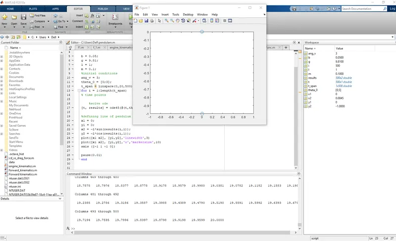
In this error, I was trying to plot the line and the marker for the pendulum differently. As a result, I was not getting the line plotted in the graph, which was solved using both in the same plot command.

The code for the ode_func function is as follows:

function [dtheta_dt] = ode_func(t,theta,b,g,l,m)

theta1 = theta(1);
theta2 = theta(2);

dtheta1_dt = theta2;
dtheta2_dt = -(b/m)*theta2 - (g/l)*sin(theta1);
dtheta_dt = [dtheta1_dt; dtheta2_dt];

end

The explanation for the code is as follows:

• The function command is used to define the function for solving dtheta_dt, which takes t, theta,b,g,l,m as its input
• theta1 theta2 are defined as theta of 1&2 to just give theta as a 2x1 array for the input.
• Then the ODEs are defined, and the result for the ODEs is obtained as dtheta_dt.