Week 3 - Solving second order ODEs

This is the code for animation of Pendulum motion.

The video link for the animation is : https://youtu.be/85D0LSlRI6w

clear all
close all
clc

%inputs
g=9.81;
L=1;
m=1;
b=0.05;
 
%initial Conditions
Omega_0=3;  %initial angular velocity rad/s

theta_0=[0;Omega_0];

%time for simulation
t_span=linspace(0,20,500);

[t, results] = ode45(@(t,theta) ode_func(t, theta, b,g,L,m),t_span, theta_0);



ct=1;
for i=1:length(t_span)
    %coordinate of the pendulam is given as
    x=-L*sin(results(i,1));
    y=-L*cos(results(i,1));

plot([0 x], [0 y],"O-","linewidth",1,"Color","r")
xlabel("X-Displacement")
ylabel("Y-Displacement")
        axis([-1.2 1.2 -1.2 -0.02])
        M(ct)=getframe(gcf);
        ct=ct+1;
end 

movie(M)
Videofile=VideoWriter("Himanshu_Pendulum_Animation.avi", "Uncompressed AVI")
open(Videofile)
writeVideo(Videofile,M)
close(Videofile)

The above code uses the function as ode_func for defining the motion equation in present analysis:

function [dtheta_dt]= ode_func(t,theta,b,g,L,m)
theta1=theta(1);
theta2=theta(2);
dtheta1_dt=theta2;
dtheta2_dt=-(b/m)*theta2-(g/L)*sin(theta1);
dtheta_dt=[dtheta1_dt; dtheta2_dt];
end 

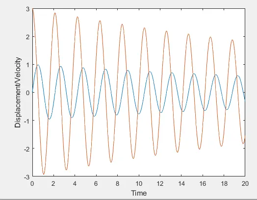
The second code prints the displacement and velocity graph on the same figure.

clear all
close all
clc

%inputs
g=9.81;
L=1;
m=1;
b=0.05;
 
%initial Conditions
Omega_0=3;  %initial angular velocity rad/s
vel_0=L*Omega_0;   %initial linear velocity m/s

theta_0=[0;vel_0];

%time for simulation
t_span=linspace(0,20,500);

[t, results] = ode45(@(t,theta) ode_func(t, theta, b,g,L,m),t_span, theta_0);

plot(t,results(:,1))
hold on
plot(t,results(:,2))
xlabel("Time")
ylabel("Displacement/Velocity")