Project 1 - Parsing NASA thermodynamic data
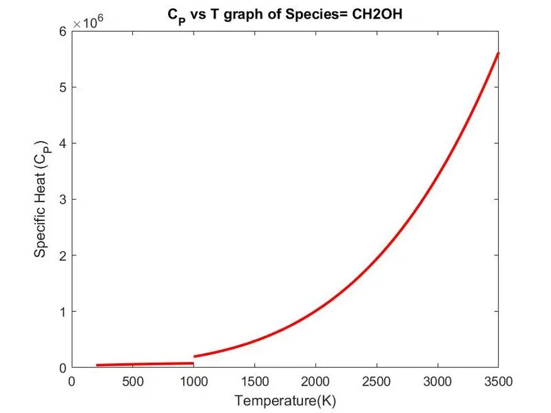
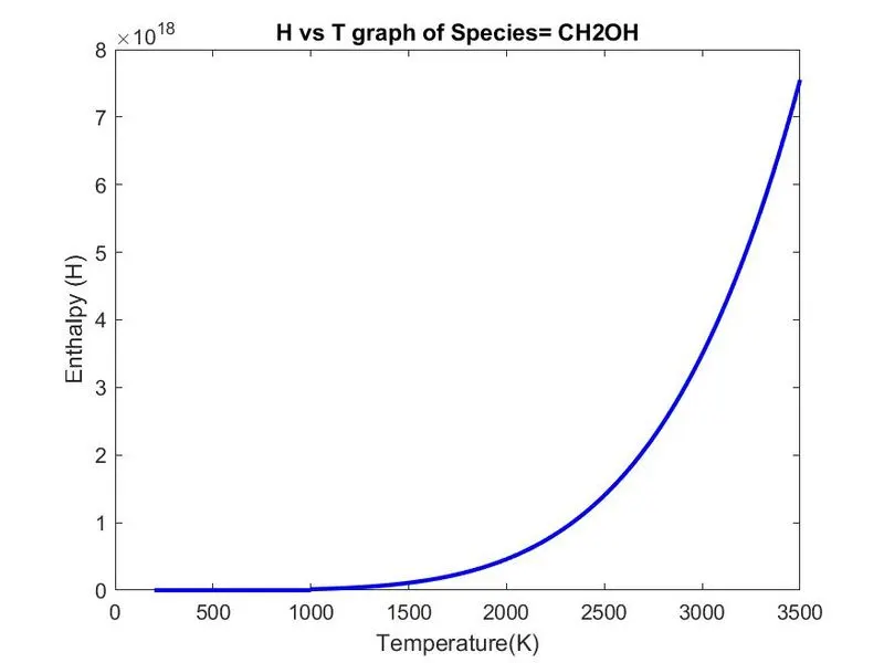
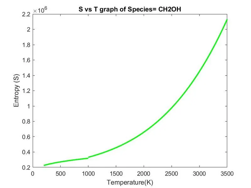
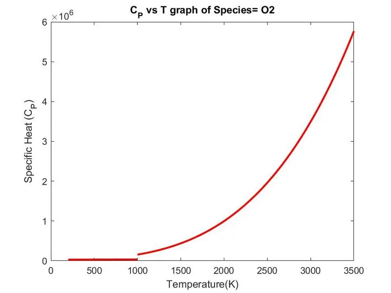
The following code will read the input file, According to the properties function, generates the properties graph wrt Temperature and saves them in a given directory for different species, Also calculate the molecular weight of the each species and print their weight in the result window.
close all
clear all
clc

% Open the file and read the file using r command
F=fopen("THERMO.dat","r");
i=1;
%declaring the Array with no. of lines as a guess
A=cell(1,220);
while 1
    A(i)={fgetl(F)};
    K=string(A(i));    % converting cell array to string
    i=i+1;
    if K=="END"        % Knowing where the end is
        break
    end
end
Num_Lines=i-1;     %Total number of lines in the given file
D=string(A(1,1:Num_Lines-1))';    %Usefull Data

%For global Temperature
tline2=strsplit(D(2)," ");
Global_min_temp=str2num(tline2(2));
Global_middle_temp=str2num(tline2(3));
Global_max_temp=str2num(tline2(4));

% Defining the species data
% Maximum 6 characters are in a species name
%Speceies name:
species_data=char(D(6:4:length(D)));   %starting from 6th line and skipping +4 lines after that

split_data=cell(53,9);
%Getting Species data
for i=1:size(species_data,1)

    Split_data(i,1:length(strsplit(species_data(i,:), " ")))=strsplit(species_data(i,:), " ");
    species(i)=Split_data(i);
end
New_species=strtrim(species);

G1=strfind(species_data(6,:),'G');     %position of G for temperature range

% Min_temp(i)=...., Medium_temp(i)=.....,Max_temp(i)=..... are the local
% temperature ranges for ith species starting from 'O' as the first species
for i=1:size(species_data,1)
    x=G1+4:size(species_data,2)-5;
    temp_data(i,1:length(x))=species_data(i,G1+4:size(species_data,2)-5);
end
temp_lim=str2num(temp_data);
%Now the temperature limits are given as:
Min_temp=temp_lim(:,1);
Max_temp=temp_lim(:,2);
Medium_temp=temp_lim(:,3);

for i=1:size(species_data,1)
    b=i-1;
   line_no(i,1:3)=[7+4*b,8+4*b,9+4*b]; % line pointer for coefficient data

%For species 1 the coefficients are determined as:
%line no. 7,8,9
%low temperature coefficient:
l1=line_no(i,1);
tline7=char(D(l1));
position1=findstr(tline7,"E");
%Low temperature coefficients
a(i,1)=str2num(tline7(2:12+3));    %starting from 2 since first element is space only
a(i,2)=str2num(tline7(12+4:27+3));
a(i,3)=str2num(tline7(27+4:42+3));
a(i,4)=str2num(tline7(42+4:57+3));
a(i,5)=str2num(tline7(57+4:72+3));

l2=line_no(i,2);
tline8=char(D(l2));
a(i,6)=str2num(tline8(2:12+3));

%high Temperature coefficients
a(i,7)=str2num(tline8(12+4:27+3));
a(i,8)=str2num(tline8(27+4:42+3));
a(i,9)=str2num(tline8(42+4:57+3));
a(i,10)=str2num(tline8(57+4:72+3));
l3=line_no(i,3);
tline9=char(D(9));
a(i,11)=str2num(tline9(2:12+3));
a(i,12)=str2num(tline9(12+4:27+3));
a(i,13)=str2num(tline9(27+4:42+3));
a(i,14)=str2num(tline9(42+4:57+3));
end

%From above loop a matrix of 53*14 will be created which will have the coefficients data
% for all the species which are there in the file

for i=1:53

%Graph for first species
%for low temperature
R=8.314*1000;               %J/k-mol universal gas constant
a1=a(i,1);
a2=a(i,2);
a3=a(i,3);
a4=a(i,4);
a5=a(i,5);
a6=a(i,6);
a7=a(i,7);
T1=Min_temp(i);
T2=Medium_temp(i);
T=linspace(T1,T2,100);
Cp=(a1+a2.*T+a3.*T.^2+a4.*T.^3+a5.*T.^4)*R;
H=(a1+a2.*T/2+(a3.*T.^2)/3+(a4.*T.^3)/4+(a5.*T.^4)/5+a6./T)*R.*T;
S=(a1*log(T)+a2.*T+(a3.*T.^2)/2+(a4.*T.^3)/3+(a5.*T.^4)/4+a7)*R;

%For High Temperature
a8=a(i,8);
a9=a(i,9);
a10=a(i,10);
a11=a(i,11);
a12=a(i,12);
a13=a(i,13);
a14=a(i,14);
TH=linspace(Medium_temp(1),Max_temp(1),100);
Cp_H=(a8+a9.*TH+a10.*TH.^2+a11.*TH.^3+a12.*TH.^4)*R;
H_H=(a8+a9.*TH/2+(a10.*TH.^2)/3+(a11.*TH.^3)/4+(a2.*TH.^4)/5+a13./TH)*R.*TH;
S_H=(a8*log(TH)+a9.*TH+(a10.*TH.^2)/2+(a11.*TH.^3)/3+(a12.*TH.^4)/4+a14)*R;


SP1=species(i);
title_graph=char(SP1);
Path="C:\Users\HKP\Documents\MATLAB\File_parsing_data";
Sub_folder=SP1;
File_Path=fullfile(Path,Sub_folder);

mkdir(fullfile(Path,Sub_folder))
cd (File_Path)

figure(1)
plot(T,Cp,"linewidth",2,"Color",'r');
hold on
plot(TH,Cp_H,"linewidth",2,"Color",'r');
xlabel("Temperature(K)")
ylabel("Specific Heat (C_P)")
title(sprintf('C_P vs T graph of Species= %s', title_graph))

saveas(gcf,"C_p_vs_T.jpeg")
hold off
close(gcf)

figure(2)
plot(T,H,"linewidth",2,"Color",'b');
hold on
plot(TH,H_H,"linewidth",2,"Color",'b');
xlabel("Temperature(K)")
ylabel("Enthalpy (H)")
title(sprintf('H vs T graph of Species= %s', title_graph))
saveas(gcf,"H_vs_T.jpeg")
hold off
close(gcf)
figure(3)
plot(T,S,"linewidth",2,"Color",'g');
hold on
plot(TH,S_H,"linewidth",2,"Color",'g');
xlabel("Temperature(K)")
ylabel("Entropy (S)")
title(sprintf('S vs T graph of Species= %s', title_graph))
saveas(gcf,"S_vs_T.jpeg")
hold off
close(gcf)
%saveas(h(k),sprintf('figure_%d.jpg',k))
cd ("C:\Users\HKP\Documents\MATLAB")

end


%For Displaying the Molecular weight of species:
%inputs required

Elements=["AR" "C" "H" "O" "N"];
Elements_weights=[40;12;1;16;14];

% Weight=0;
species_char=char(species);

for k=1:53
Weight=0;
for i=1:6
hg=species_char(k,i);
m=0;
p=0;
for j=1:5
    hg;
if hg==Elements(j)
Weight=Weight+Elements_weights(j);
pos=j;
end
hh=species_char(k,1:2);
if p==0
if hh==Elements(j)
Weight=Weight+Elements_weights(j);
p=p+1;
end
else
    Weight=Elements_weights(1);
end
if m==0
pm=str2num(hg);
else
    pm=0;
end
if pm>=1
Weight=Weight+Elements_weights(pos)*(pm-1);
m=m+1;
end

end
end

fprintf("molecular weight of species no. %1.0f, %s = %4.1f \n",k,species_char(k,1:6),Weight)
end
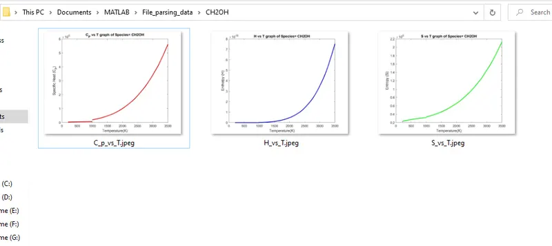
This is the screenshot of files saved in a directory with folder names
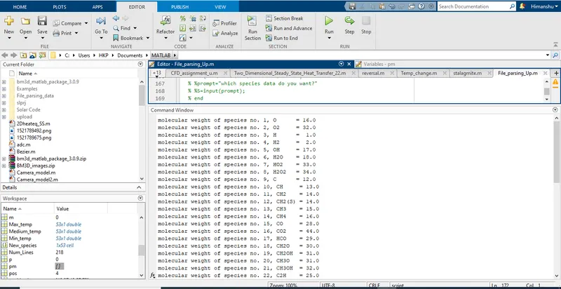
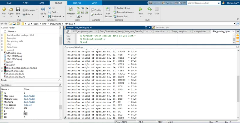
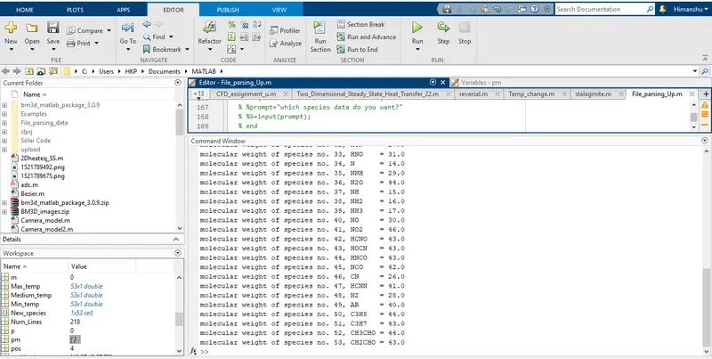
The above screen shot is the molecular weight calculation using the following code:
%For Displaying the Molecular weight of species:
%inputs required

Elements=["AR" "C" "H" "O" "N"];     %Elements names
Elements_weights=[40;12;1;16;14];    %Corresponding elements weights

% Weight=0;
species_char=char(species);

for k=1:53
Weight=0;
for i=1:6
hg=species_char(k,i);
m=0;
p=0;
for j=1:5
    hg;
if hg==Elements(j)
Weight=Weight+Elements_weights(j);
pos=j;
end
hh=species_char(k,1:2);
if p==0
if hh==Elements(j)
Weight=Weight+Elements_weights(j);
p=p+1;
end
else
    Weight=Elements_weights(1);
end
if m==0
pm=str2num(hg);
else
    pm=0;
end
if pm>=1
Weight=Weight+Elements_weights(pos)*(pm-1);
m=m+1;
end

end
end

fprintf("molecular weight of species no. %1.0f, %s = %4.1f \n",k,species_char(k,1:6),Weight)
end
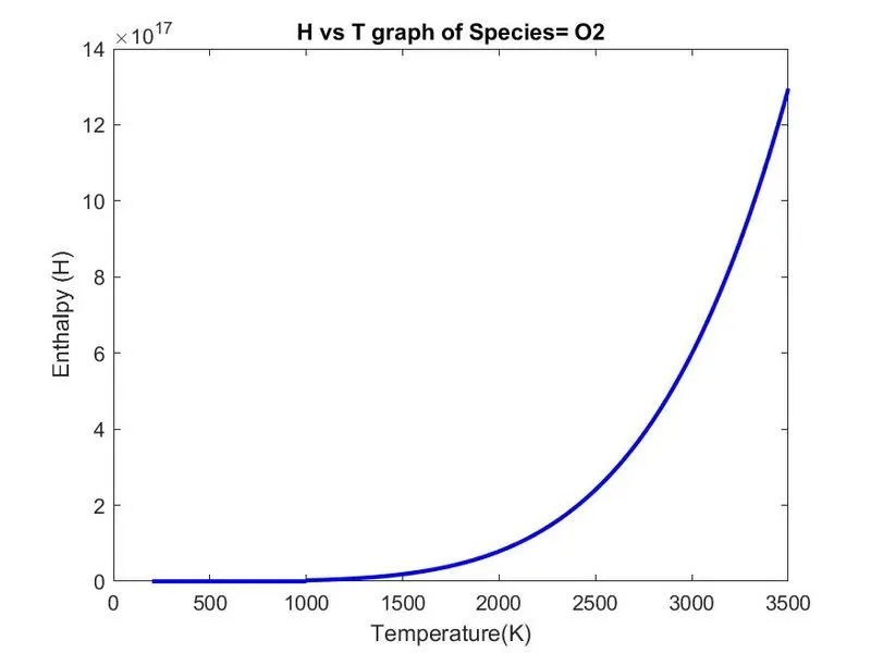
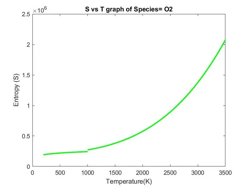
Plots for O2:
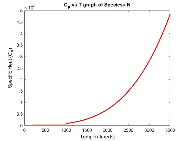
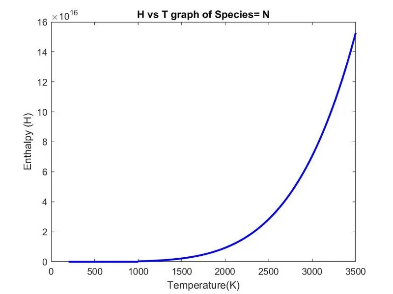
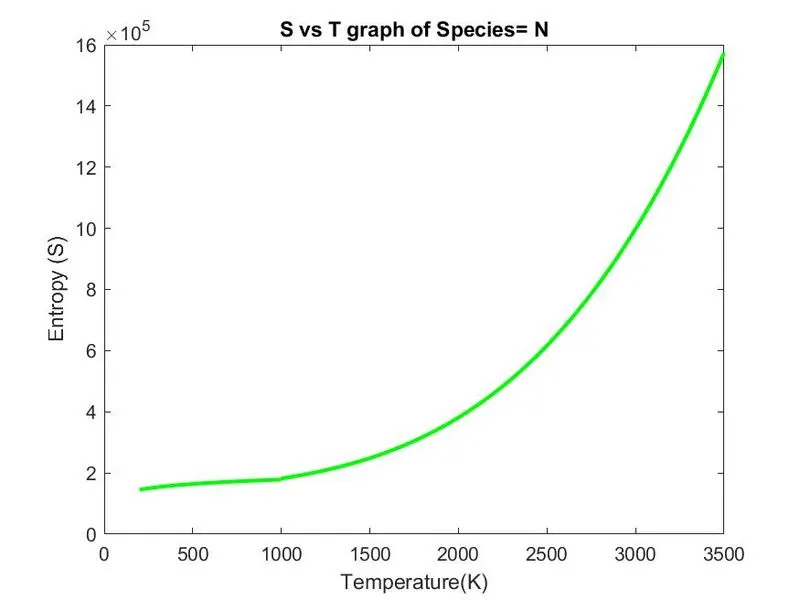
Plots for N2
Plot of CO2
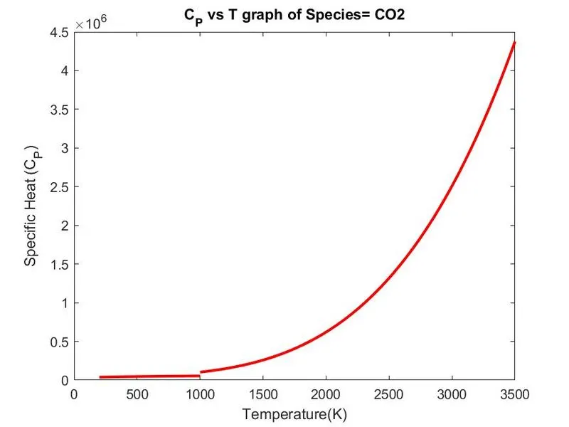
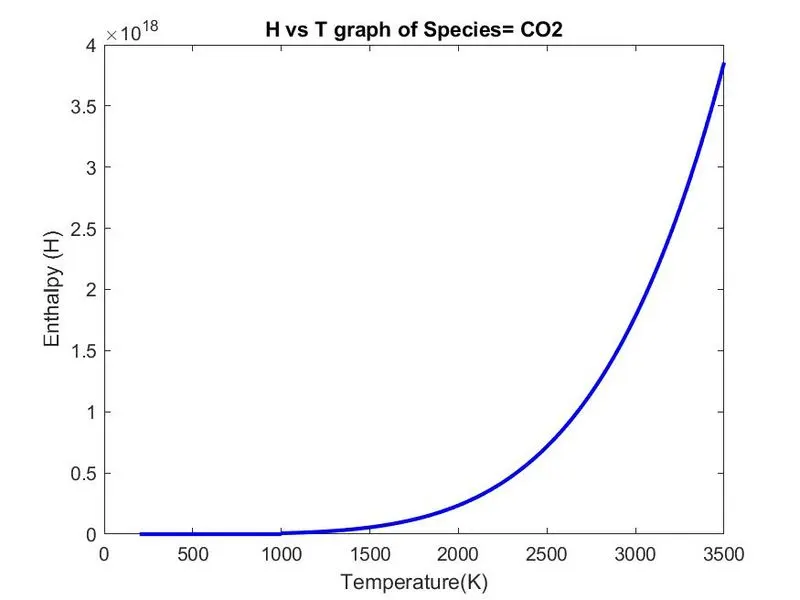
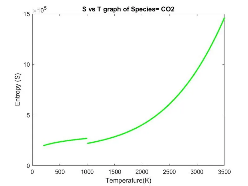
Explaination: The code has been written in accordance to the given file structure and pattern.
The pattern of the different species data is analyzed by opening the file in a notepad. When different species pattern is understood then using fgetl command different lines are imported into a cell array and this cell array is converted to a string array and using strsplit command, different constants are acquired into the respective species data and then low temerature and high temperature ranges are also calculated. Based in the temp range and the equation for properties has been applied and then the calculation of peropertie at different temp ranges is done and plots are generated with peoper labela and title for each properties.
Now the molecular weight are also calculated using a seperate code consisting of multple for and if statements. It is done to get the correcte value of the weight so that no derepencies are there. The weight of Known elements are given in a matrix. Also the elements name matrix is also developed for comparing the species with the proper elements name. and hence the weight is determined.
Refrences:
https://in.mathworks.com/matlabcentral/answers/7164-using-and-operator-in-if-statements