Week 3 - Solving second order ODEs

The given task is to simulate pendulum motion in MATLAB/Octave, I have used MATLAB to do this.

This ODE represents the equation of motion of a simple pendulum with damping.

 `(d^2θ)/(dt^2)+(b/m)⋅(dθ)/dt+(g/l)⋅sin(θ)=0`

As this is a second-order ODE, we need to simplify it into two first-order ODE's

for this, we introduce two variables: `θ_1,θ_2`

`θ=θ_1` ----> 1

`(dθ)/dt=(dθ1)/dt=θ_2` ---->2

hence, `(d^2θ)/dt^2=d/dt((dθ)/dt)=d/dt((dθ_1)/dt)=(dθ_2)/dt` ---->3

Substituting 1,2,3 in the main ODE, we get

`(dθ_2)/dt+b/m⋅θ_2+g/l⋅sin(θ_1)=0`

`(dθ_2)/dt=−(b/m*θ_2)−(g/l⋅sin(θ_1))` ----->4

We use equations 2 and 4 to make a function and use it in the ode45 solver.

The following code was used to obtain the result; every important step is explained in detail.

%pendulum Equation is a second-order equation; we split the second-order equation into two first-order equations

%time 0-20 sec, angular displacement=0,angular velocity= 3 rad/sec2 at time t=0.

close all
clear all
clc

t = 0:0.05:20; %0-20s for every 0.05 seconds
theta0 = [0 3]; %Angular Displacement = 0, Angular velocity =3, initial conditions at t = 0

%input values, taken here for the ease of changing 

b=0.05; %damping coefficient
g=9.81; %acceleration due to gravity (m/s^2)
m=1; %mass (kg)
l=1; %length (m)

%calling the Ode45 function used the anonymous function command because we take the values of b,g,m,l from the main code.

[t,theta] = ode45(@(t,theta) pendulum_function(t,theta,b,g,m,l),t,theta0)

%used subplot function for aesthetics and ease of representation.

subplot(2,1,1)
plot(t,theta(:,1),'r')
xlabel('Angular Displacement (rad)')
ylabel('time (s)')
grid on
subplot(2,1,2)
plot(t,theta(:,2),'k')
xlabel('Angular velocity (rad/s)')
ylabel('time (s)')
grid on


% following For loop was used to plot the position of pendulum bob at every instance

count = 1;  %initializing counter
for i=1:length(theta)
    angle = theta(i,1); 
    x0=0; %defining origin position
    y0=0;
    x1=l*sin(angle) %defining position of bob in cartesian plane
    y1=-l*cos(angle)
    figure(2)
    plot(x1,y1,'o','markersize',20,'markerfacecolor','b')
    hold on
    plot([x0 x1],[y0 y1],'linewidth',2,'color','c') %plotting the sstring
    plot([-1 1],[0 0],'linewidth',10,'color','k') %plotting the beam
    axis ([-1.5 1.5 -1.5 .5]) %defining axis to maximize the view of pendulum
    hold off
    M(count)=getframe(gcf); %capturing each frame
    count=count+1;
    
end

%following code is to stitch the frames and make an AVI video file.

movie(M)
videofile = VideoWriter('simplependulum.avi','Uncompressed AVI');
open(videofile)
writeVideo(videofile,M)
close(videofile)​

Function:

function [theta_dot] = pendulum_function(t,theta,b,g,m,l);

theta_dot = zeros(2,1)
theta_dot(1) = theta(2);
theta_dot(2) = -(b/m)*theta(2) - (g/l)*sin(theta(1));
end

The Resulting Graph

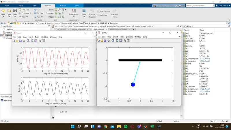
The Video