Week 3 - Solving second order ODEs

% simple pendulam and ode function


clear all
close all
clc

b=0.05;
l=1;
g=9.81;
m=1;

%intial condition 
x=[0;3];

%time 
time=linspace(0,20,150);

%solve ode
[t,output]=ode45(@(t,x) ode_func(t,x,b,g,l,m),time,x)
%plot for angular velocity and angular displacement
plot(t,output(:,1),'lineWidth',2,'color','black')
hold on
xlabel('time');
ylabel('angular displacement')
plot(t,output(:,2),'linewidth',2,'color','blue')
% animatin

x0=0;
y0=0;
theta=output(:,1)
ct=1;
for i=1:length(theta)
    x1=l*sin(theta(i));
    y1=-l*cos(theta(i));

    
    figure (2)
    plot([-1 1],[0 0],'linewidth',3,'color','r');
    axis([-2 2 -2 2])
    line([x0 x1],[y0 y1],'linewidth',2,'color','b');
    hold on
    plot(x0,y0 ,'o','markersize',1,'markerfacecolor','y');
    plot(x1,y1,'o','markersize',20,'markerfacecolor','g');
    title('damping of simple pendulam')
    legend('supportrod','length of pendulam','fixed point','pendulam');
    hold off
    pause(0.5);
    M(ct)=getframe(gcf);
    ct=ct+1;
end
movie(M)
Videofile = VideoWriter('pendulam.avi','uncompressed AVI');
open(Videofile)
writeVideo(Videofile,M)
close(Videofile)

%% ode function

function[dx_dt]=ode_func(t,x,b,g,l,m)
x1=x(1)
x2=x(2)
dx1_dt=x2;
dx2_dt=-(b/m)*x2-(g/l)*sin(x1);
dx_dt=[dx1_dt;dx2_dt];
end

explanation:

step1:i take some values damping coefficient,length of pendulam,gravity,mass given in challenge question

step2:intially i take x=[0;3]; 0-angular displacement,3=angular velocity

step3:time=linspace(0,20,150) take time values between 0 to 20 with 150 values same interval by using linspace command

step4: function[dx_dt]=ode_func(t,x,b,g,l,m) here we assume theta=x and using fomula given in challange
x1=x(1)=>angular displacement
x2=x(2)=>angular velocity
dx1_dt=x2;
dx2_dt=-(b/m)*x2-(g/l)*sin(x1);
dx_dt=[dx1_dt;dx2_dt];

step5:here we use ode45 (inbuilt function ) and @ -it is calling function

[t,output]=ode45(@(t,x) ode_func(t,x,b,g,l,m),time,x)

t is time span and output values

step6:

here we plot time and output(all rows and angular displacement values)

plot(t,output(:,1),'lineWidth',2,'color','black')

step7:

here we plot time and output(all rows and angular velocity values)

plot(t,output(:,2),'linewidth',2,'color','blue')

step8:

theta=output(:,1) here we take theta=output of all rows and angular displacement values

step9: here we use for loop

for i=1:length(theta)=> 1 to 150 values (all rows and angular displacement because calucalate the values for time and angular displacement
x1=l*sin(theta(i));=> angular displacement in radian values
y1=-l*cos(theta(i));=>angular displacement in radian values

step9: we plot support rod

plot([-1 1],[0 0],'linewidth',3,'color','r');

length of pendulam

line([x0 x1],[y0 y1],'linewidth',2,'color','b');

plot pendulam bob(sphere) by using marker command

plot(x0,y0 ,'o','markersize',1,'markerfacecolor','y');
plot(x1,y1,'o','markersize',20,'markerfacecolor','g');

finally i run my programm and animation was done .by using movie commands save in my folder

youtubelink for simple pendulam animation:https://youtu.be/VYiz-3YIPto

ERRORS:

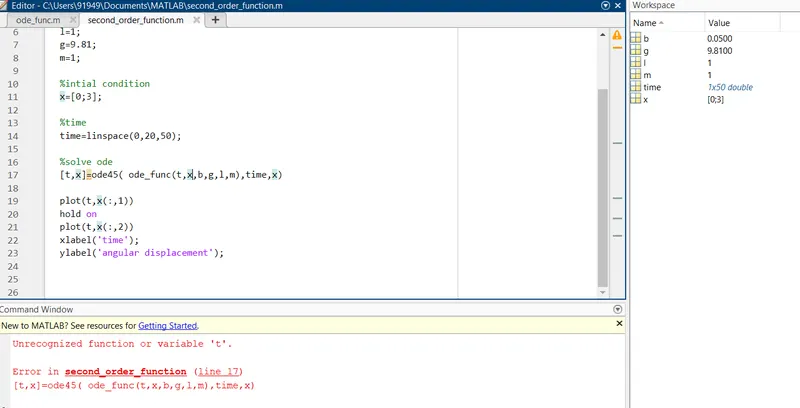
here i forgot t values in ode function

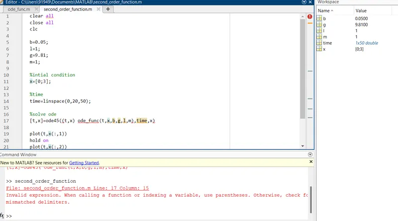
here @-calling function

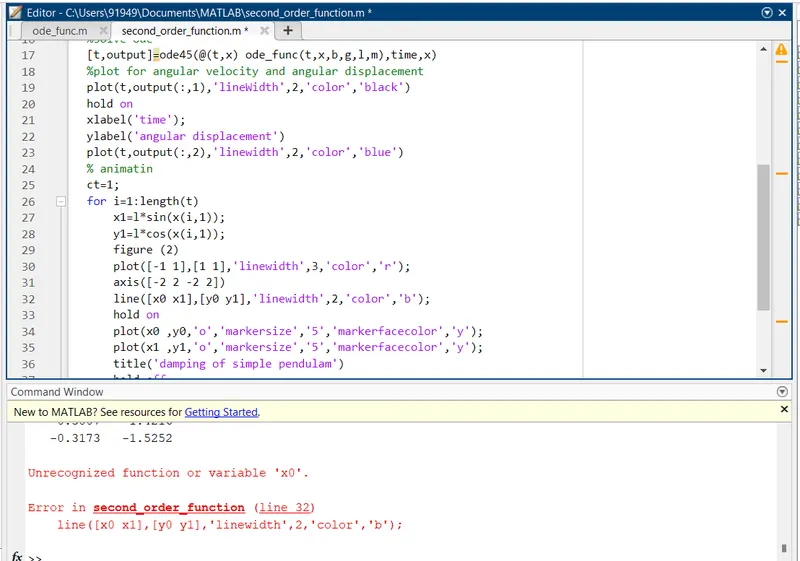
here i forgot coordinates x0=0,y0=0 and in for loop length(t) but t value given then i got we take the angular displacement values so for i= 1 to lenngth(angular displacememt values)

then we take theta =output(:,1)

fori=1:length(theta) and x1= l*sin(theta(i) )same as y1=l*cos(theta(i))