Week 3 - Solving second order ODEs
Aim:-
To simulate a simple pendulum by solving second-order Ordinary Differential
Equation with the help of MATLAB.
Objectives:-
● Solve the second-order Ordinary Differential Equation.
● to create an animation file of a pendulum.
● to simulate the motion between 0-20 sec, for angular displacement=0,angular
velocity=3 rad/sec at time t=0.
Solving Second-order Ordinary Differential Equation:-
The given equation represents the equation of a simple pendulum.
In the above equation,
g = gravity in m/s2,
L = length of the pendulum in m,
m = mass of the ball in kg,
b=damping coefficient.
To convert this second order Ordinary Differential Equation to first order Ordinary
Differential Equation.
let,
dθdt=dθ1dt=θ2------(1)
d2θdt2=d2θ1dt2=ddt(dθ1dt)=ddt(θ2)-----(2)
d2θdt2+bm⋅dθdt+gl⋅sin⋅(θ)=0
d2θ1dt2+bm⋅dθ1dt+gl⋅sin(θ1)=0
dθ2dt+bmθ2+gl⋅sin(θ1)=0
dθ2dt=-bm⋅θ2-gl⋅sin(θ1)
After solving this equation we can solve this equation in MATLAB, the programing to
solve this equation of pendulum is given below.
MATLAB Program:-
For Function equation:-
function [dtheta_dt] = ode_func(t, theta, b, g, l, m)

theta1 = theta(1);
theta2 = theta(2);

dtheta1_dt = theta2;
dtheta2_dt = -(b/m)*theta2 -(g/l)*sin(theta1);

dtheta_dt = [dtheta1_dt ; dtheta2_dt];

end
Explanation:-
● This program is used to create the values dtheta_dt in matrix form so that we can
use these values to calculate the values of angular velocity and angular
displacement.
● Here we use the function command to find the values of dtheta _dt with the help
of formula [dtheta_dt] = ode_func(t,theta,b,g,l,m) .
● We can call this code to our main code to find the values of angular displacement
and angular velocity with the help of this function command.
● dtheta1_dt = theta2; dtheta2_dt = -(b/m)*theta2 - (g/l)*sin(theta1); dtheta_dt =
[dtheta1_dt; dtheta2_dt]; this formulas can be used to get the values of dtheta_dt.
● After this program, we wrote the main program code which is given below.
For Pendulum:-
close all
clear all
clc

b = 0.05;
g = 9.81;
l = 1;
m = 1;

% initial condition %
theta_0 = [0;3];

% time points %
t_span = linspace(0,20,200);

% solve ODE %
[t, results] = ode45(@(t,theta) ode_func(t,theta,b,g,l,m),t_span, theta_0);

% plotting for angular velocity and displacement %
figure(1)
title('motion of pendulum')
plot(t,results(:,1))
hold on
plot(t,results(:,2))
ylabel('angular velocity (rad/s)/ displacement (rad)')
xlabel('time (sec)')
legend('displacement','angular velocity')

angle = results(:,1);

ct = 1
for i = 1:length(angle);
    omega = angle(i);

    figure(2)
    % fixed coordinates of one end of pendulum
    x0 = 0;
    y0 = 0;
    % free end coordinates
    x1 = l*cos((3*pi/2)+omega);
    y1 = l*sin((3*pi/2)+omega);

    % bob motion
    plot([x0 x1],[y0 y1],'linewidth',3,'color','g')
    hold on
    plot(x1,y1,'O','markers',15,'markerfacecolor','r')
    hold on
    plot([-2 2],[0 0],'linewidth',2,'color','k')
    hold off
    axis([-2 2 -2 2])
    grid on
    M(ct) = getframe(gcf)
    ct = ct+1;
end

% creating video file %
movie(M)
Videofile = VideoWriter('simple pendulum.avi')
open (Videofile)
writeVideo(Videofile,M)

close(Videofile)
Explanation:-
● First, we use the clear all, close all, and clc commands to clear all the unwanted
data in the workspace and the command window and close background plots.
● After that, we provide all the necessary input data to the program which is
L=1 meter,
m=1 kg,
b=0.05.
g=9.81 m/s2
● Also, we provided the initial condition of angular displacement=0, angular
velocity=3 rad/sec at time t=0 to simulate the motion between 0-20 sec.
● While providing input data, we used linspace to generate an array of t_span from
0 to 20 sec of 500.
● To solve the second-order Ordinary Differential Equation we use the ode45
command where we called function equation from ode_fun from function code as
we mentioned earlier.
● With the help of this command, we find the values of [t, result] which we can use
to plot the movement of the pendulum with respect to its angular velocity and
angular displacement.
● To plot the plot of angular velocity and angular displacement we use the plot
command first we plot angular displacement using the plot command
plot(t,result(:,1)) then we used hold on command to stop overwriting of this curve
over another curve.
● And to plot angular velocity we used plot(t,result(:,2)) then we use xlabel and
ylabel commands to give names to the x and y-axis as time and plot respectively.
● Then title command is used to name the plotted graph as pendulum
displacement.
● To make an animation of the pendulum we used counter command and a for loop
command in for loop I variable is used to 1:length(t) to get the time values which
can be used to find the values of x and y variable.
● Then to plot a pendulum we used plot command as plot([-1,1],[0,0],'linewidth',5)
with this we are able to plot the horizontal bar of a pendulum, and for the vertical
bar we used plot([0,x],[0,y],'linewidth',5) within this command we used hold on
command to stop overwriting the plot command hold off command is used after
that.
● plot(x,y,'Marker','o','Markersize',25,'Markerfacecolor','r') is used to plot the circular
shape of a pendulum with all this we successfully plot our pendulum with
animation.
● To give the pendulum a fixed motion we used the axis command at a point
axis([-1.5,1.5,-2,2]);
● title command is used to name the figure as a pendulum.
● M(ct) command is used after a pause command to capture the current frame
every time for 'for loop'.
● The code ct=ct+1 is used for incrementing the frame every time the for loop runs.
● After that, we end the for loop using the end command.
● And in the end, to make a video of the plotting of a pendulum we used the movie
command after that video file command is used where 'pendulum_movement' is
the name of the video which is about to save in the device and 'Uncompressed
AVI' is the file type.
● The open command is used to open the video and the WriteVideo command is
used to write plots in a video format after that close command is used to close
the video.
● After writing this we used the run button which is in the taskbar or use f5 to run
the program.
● With the help of the above codes, we get our pendulum in video formal as an
output successfully.
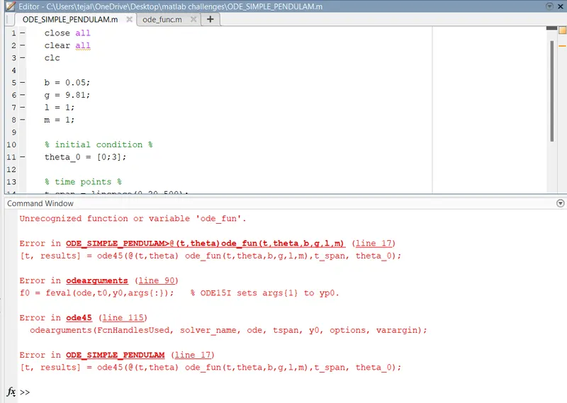
errors:-
Youtube link for the simple pendulum:-