Week 3 - Solving second order ODEs
%example:d2o/dt+b/m. do/dt +g/l . sino
clear all
close all
clc
theta0=[0;3];%given conditions of angular velocity from 0 to 3m/s
L=1;%length of rope of pendulum is 1m
t_span =linspace(0,20,100);%given time is start at 0s to 20s ,interval of time is decided by user i.e100 intervals.
[t, results] = ode45(@(t,theta) dampingpendulum(t, theta,L), t_span, theta0);
% ode 45fuct is inbuilt funct. of matlab , it allows 2 inus and solves
% problems only in 1st order differential eqs . @ sign tells the functn
% that t, theta are the main inputs of the funct.
x0=3;%stating the initial conditions i.e origin of pendulum x0 y0
y0=3;
ct=1;%count of figures is initialise to 1
displacement=results(:,1); %the results stored in results, 1st column is given specific location to store i.e displacement
velocity=results(:,2);%the results stored in results, 2nd column is given specific location to store i.e velocity
figure(101)%for the plot of (t,disp,and vel graph)
%plot(t,displacement)
plot(t,displacement,'r<--') %the graph will be shown in dotted line with arrow indicating backwards with in red
hold on
%plot(t,velocity)
plot(t,velocity,'k->')%the graph will be shown in dotted line with arrow indicating forward with in black
legend('displacement in theta','Velocity in m/s') %displaying the meaning of lines
grid on
hold off
for i=1:length(displacement) % since it has been given initial velocity from free, we req. for loo for every action or disp. of theta-
%-it is going from 0 to t sec.
Theta=displacement(i);%theta is aligned with disp. as i changes , theta changes
figure(ct);%figure is captured from i=1 to length of disp.column
hold on
x= x0+ L*sin(Theta); %position of x and y changes as value of theta changes
y=y0-L*cos(Theta);
% plot(x,y,'r<--')
PLOT=plot ([x0 x], [y0 y]);%plotting of x0 x and y0 y coordinates which forms a roe of endulum for various values of theta
plot(x0,y0 ,'s','Markersize',5)%origin og rope to which pendulum is hinged to wall
plot(x,y ,'.','Markersize',50)% pendulum
axis([1.5 4.5 1 4])%x axis varies from 1.5 to 4 anf axis varies from 1 to 4
text (x0,y0,'origin')%shows the 'origin' in text
hold on
grid on
pause(0.1)
m(ct)=getframe(gcf)%storing the frames tillthe length of disp.
ct=ct+1;%increment of count
end
movie(m) %defining movie
videofile=VideoWriter('damping.avi','uncompressed AVI')%the movie must be in uncompressed form
open(videofile)
writeVideo(videofile,m)%the data collected by m(ct) is used to cresate the mvie or animation
close(videofile)
%function call
function [dtheta_dt] = dampingpendulum(t, theta,L)
m = 1;%given mass is 1kg
g = 9.81;%acc. due to gravity 9.81m/s
b=0.05;%damping coeff 0.05
theta1 = theta(1); % eqn solver, o is reffered as theta ;o=o1,d0/dt=d01/dt=o2 i.e vel
%d2o/dt2=acc.=d/dt (do/dt)=d/dt(o2)
theta2 = theta(2);
dtheta1_dt = theta2;
dtheta2_dt =-b/m * theta2-g*sin(theta1)/L ;% the above exmle has been converted to 1st order diff eqn.
dtheta_dt = [dtheta1_dt;dtheta2_dt];
end
%errors faced;
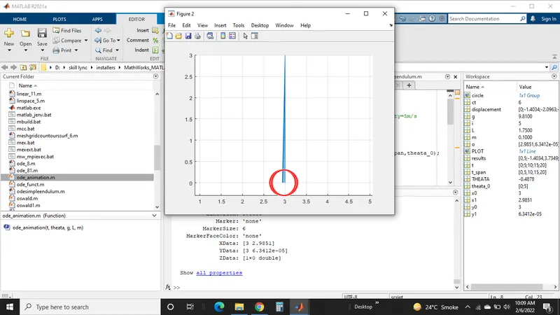
1. pendulum was getting overlaed imaged is attached below . soln was rewriting the program along with rectification .. in the imaged i have used viscircle command insted of marker command.
2.the main graph was getting overlaped in the animation of pendulum. sol. i had interfaced the ct value.
youtube link as been attached below