Week 3 - Solving second order ODEs

AIM:

    To write a program that solves the second order differential equation. 

GIVEN:

     In Engineering, ODE is used to describe the transient behavior of a system. A simple example is a pendulum

     The way the pendulum moves depends on the Newtons second law. When this law is written down, we get a second order Ordinary Differential Equation that describes the position of the "ball" w.r.t time. 

     Similarly, there are hundreds of ODEs that describe key phenomena and if you have the ability to solve these equations then you will be able to simulate any of theses systems.

     

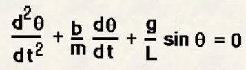
In the above equation,

g = gravity in m/s2,
L = length of the pendulum in m,
m = mass of the ball in kg,
b=damping coefficient.

OBJECTIVE:

     To write a program in Python that will simulate the pendulum motion.

• L=1 metre,
• m=1 kg,
• b=0.05.
• g=9.81 m/s2.
• time =0-20 sec
• Angular displacement=0,
• angular velocity=3 rad/sec at time t=0.

SOLUTION:

     Now, lets open sublime and create a program in python that will simulate the pendulum motion.

PYTHON PROGRAM:

# Program to simulate the simulate the pendulum motion.

# importing essential library tools
import math                         # importing math library
import matplotlib.pyplot as plt     # importing ploting library
import numpy as np                  # importing computing library
from scipy.integrate import odeint  # importing ODE library

# function definiton
def model(theta,t,b,g,l,m):  # defining the model of the system in function
	theta1=theta[0]  
	theta2=theta[1]
	dtheta1_dt=theta2
	dtheta2_dt= -(b/m)*theta2-(g/l)*math.sin(theta1)  # ODE equation
	dtheta_dt=[dtheta1_dt,dtheta2_dt]
	return dtheta_dt

# Input parameters
b=0.05  # damping coefficient
g=9.81  # Gravity
l=1  # length of the pendulum
m=1  # mass of the pendulum

# initial condition
theta_0=[0,3]  # Angular displacement and angular velocity.

# Time space
t=np.linspace(0,20,150)  # time stamp of 0 to 20 secs.

# computing ODE
theta=odeint(model,theta_0,t,args=(b,g,l,m)) # calling the ODE equation

# Plotting
plt.plot(t,theta[:,0],'b--',label=r'$\frac{d\theta_1}{dt}=\theta2$')  # plotting the angular displacement
plt.plot(t,theta[:,1],'r--',label=r'$\frac{d\theta2}{dt}= -\frac{b}{m}\theta_2-\frac{g}{l}sin\theta_1$')  # plotting the angular velocity
plt.grid()  # turning the grids on
plt.title('')  # labeling the title
plt.xlabel('Time')  # labeling the x axis
plt.ylabel('Displacement')  # labeling the y axis
plt.xlim([0,12])  # limiting the x axis
plt.legend(loc='best')  # legend
plt.show()  # displaying the plot

# Simulation of simple pendulum
T3=[]  # user defined constant
for theta3 in theta[:,0]:  # declaring theta3 in loop
	T3.append(theta3)  # attaching T3 in the loop
ct=1  # point of contact

for T4 in T33:  # declaring t4 in loop
	x0=0  # point at wall
	y0=0  # point at wall

	x1=l*math.sin(T4)  # movement of the bob
	y1=-l*math.cos(T4)  # movement of the bob

	
	filename=str(ct)+'.png'  # saving the image in png
	ct=ct+1  # incrementing the contact point

	# plotting for simulation

	plt.plot([-0.2,0.2],[0,0])  # ploting the fixed point damper
	plt.plot([x0,x1],[y0,y1])  # ploting the string
	plt.plot(x1,y1,'-o')  # ploting the bob
	plt.xlim([-1.5,1.5])  # limiting x axis
	plt.ylim([-1.5,1])  # limiting y axis
	plt.title('simulation of pendulum')  # title for the figure
	plt.savefig(filename)  # saving the file name
	
# end

EXPLANATION: 

• STEP 1: importing essential library tools.
  
  • importing all the neccessary librbary tools lke math, matplot.lib,numpy.
  • for ode operation tools we will importing the ODE library from scipy.integrate.
• STEP 2: Defining the function.
  
  • in this step we will be defining the function for the model, like time, damping coefficient, gravity, length and mass.
  • using retrun command the values will be returned to ODE.
• STEP 3: Input parameters.
  
  • definig the damping coefficient, gravity, length and mass as per the objectives given.
  • declaring initial conditions with anglular velocity and angluar dispalcement and declaring the time factor also as per the objective given.
• STEP 4: plotting for ODE.
  
  • for plotting we will ne using plt.plot command, for plotting the angular displacment we will be using theta value till 0, and for angular velocity we will differentiating velocity to get displacement. followed by labeling axis, titleing and legend.
• STEP 5: Simulation of simple pendulum.
  
  • initially we will be using a user defined constant, and will be declaring theta in the loop along with te variable.
  • then, we will be attaching T3 in the loop and assigning contact point as 1.
  • then we will be decalring t4 in the loop and fixing point as x0=0,y0=0.
  • Next we will be giving expressions for the movement of the bob inorder to swing.
  • Saving the file in string and incrementing the contact point.
• STEP 6: plotting for simulation.
  
  • first we will be plotting the fixed point for damper, then plotting the string, plotting the bob and limitng x and y axis and giving the title.

OUTPUT:

     

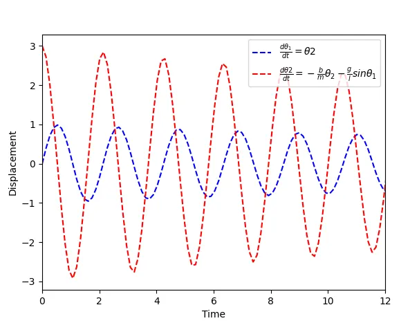
• the above graphs tells us about time and displacement.
• as per the objectives given in the question.
• the the displacement starts at 3 and represented in red colour.
• the differentiation of velocity in displacement and displacement starts at 0.
• so we can understand the pendulum oscillates sinusoidally.

     

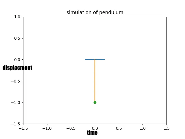
• this figure shows the simulation of the simple pendulum as per the program.

ERRORS:

• SyntaxError: 'return' outside function.
• ModuleNotFoundError: No module named 'odeint'
• NameError: name 'theta_o' is not defined.
• AttributeError: 'float' object has no attribute 'g'
• UnboundLocalError: local variable 'dtheta_dt' referenced before assignment
• ValueError: Unrecognized character 0 in format string
• ValueError: \frac{d\theta_2}{dt}=\frac{b}.{m}\theta_2-\frac{g}{l}sin\theta_1

RESULT:

     Thus the program that solves the second order differential equation is completed successfully and simulation of the pendulum is also completed and the output is verified.