Week 3 - Solving second order ODEs
Objective -
To solve 2nd ODE representing pendulum motion with damping. The governing equation is as below
Simple Pendulum-
A simple pendulum consists of a bob and a massless rod in which one end is pivoted. When the bob is given an initial angular velocity, the bob starts moving to and fro motion then comes to mean position after some time due to damping. More is the damping coefficient, sooner the stability is achieved.
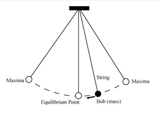
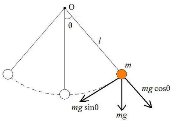
The governing equation of simple pendulum motion is as below
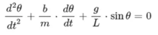
where
m = mass of the bob
L = length of string/rod
g = acceleration due to gravity
b = damping co-efficient
θ = angle of displacement, θ is a function of time
Above 2nd ODE can be simplified to 1st ODE by assuming
θ = θ1
dθ/dt = θ2
Hence it can be further converted to
dθ/dt = dθ1/dt = θ2 -----------(eqn1)
θ2 represents 'Angular Displacement'
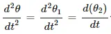
Putting the above expression in the main governing equation
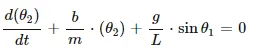
=> dθ2/dt = (-b/m) θ2 - (g/l)sinθ1 -------------(eqn2)
dθ2/dt represents 'Angular Velocity'
From eqn1 & eqn2,
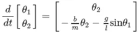
Initial conditions are given as
At t=0,
Angular displacement =0
Angular Velocity = 3 rad/sec
The timespan of 20 sec have to be calculated
Considering the given value
m=1 kg
l=1m
b=0.05
g=9.81m/s2
This simple ODE can be solved through MATLAB.
Program#1#plottings & Animation
% To solve 2nd ODE for pendulum motion

%%Inputs (all in SI units)
%mass of the bob(kg)
m=1;
%length of rod(m)
l=1;
%Damping coefficient
b=0.05;
%Acceleration due to gravity(m/s^2)
g=9.81;

%%Time span
t_span = linspace(0,20,200);

%%Initial condition at t=0(Angular disp = 0, Angular velocity = 3 rad/s)
theta_0 = [0,3];

%%ODE Solving
[t,results] = ode45(@(t,theta) ode_func(t,theta,b,g,l,m), t_span,theta_0);
Angular_disp = results(:,1);
Angular_vel = results(:,2);
%%Plottings

figure(1)
hold on
plot(t, Angular_disp)
plot(t, Angular_vel)
xlabel('time');
ylabel('Angular disp & Angular Velocity')


%%Animation - pendulum swing
figure(2)
x0=0;
y0=0;

ct=1

for i = 1 : length(Angular_disp)
    x1 = (l*sin(Angular_disp(i)));
    y1 = -(l*cos(Angular_disp(i)));


    plot([-0.5 0.5],[0 0],'LineWidth',3,'Color','b')
    hold on
    plot([x0 x1],[y0 y1],'LineWidth',2,'Color','g')

    plot(x1,y1,'*','markersize',25,'Color','r');
    axis([-2 2 -2 2]);

    hold off
    M(ct)=getframe(gcf);
    ct = ct+1

end

movie(M)
Videofile = VideoWriter('Simple_pendulum.avi','Uncompressed AVI')
open(Videofile)
writeVideo(Videofile,M)
close(Videofile)
Program#2 - For defining the function
%%Function to solve

function [dtheta_dt] = ode_func(t,theta, b,g,l,m)
theta1=theta(1);
theta2=theta(2);

dtheta1_dt = theta2;
dtheta2_dt = -((b/m)*theta2) - ((g/l)*sin(theta1));

dtheta_dt = [dtheta1_dt;dtheta2_dt]

end
Results -
By use of this MATLAB program 2nd ode for pendulum motion is solved for the given inputs& simulates angular displacement & angular velocity function with time for given damping coefficient & the below graph shows the same for a time span of 20 secs.
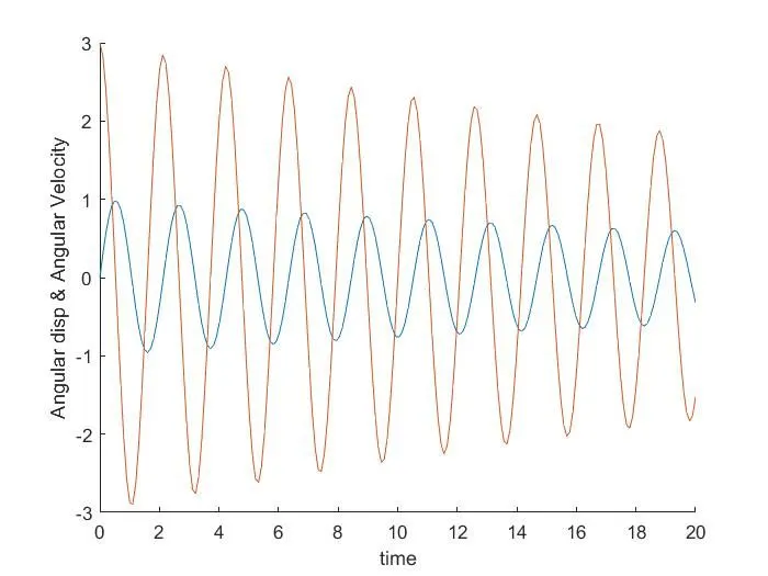
Blueline - Angular displacement (starts from the origin as initial displacement = 0)
Redline - Angular velocity (As initial value put = 3 rad/s)
Complilation -
Results –
>> Assignment6
dtheta_dt =
3.0000
-0.1500
dtheta_dt =
3.0000
-0.1504
.
.
.
dtheta_dt =
-1.5252
3.1370
ct =
1
ct =
2
.
.
.
.
ct =
199
ct =
200
ct =
201
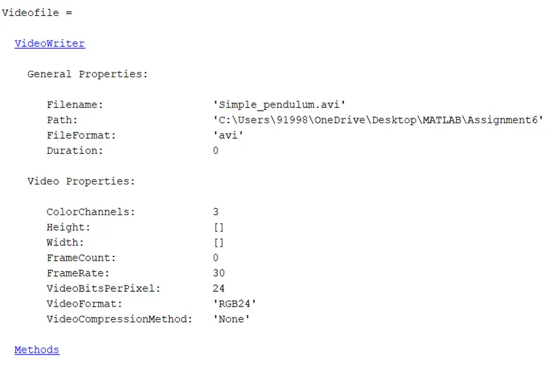
Simple pendulum model compiled as below
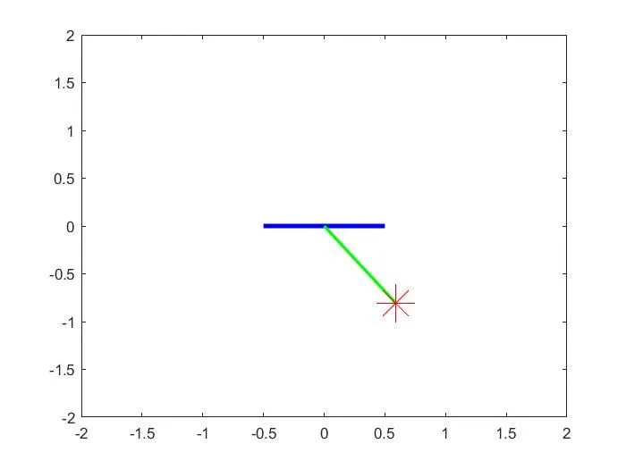
Greenline represents massless rod/string & red marker point represents the bob.
The attached ODE_Solve_explanation.pdf file shows the stepwise explanation of the code as well as the error faced.
Below is the link for animation created for a simple pendulum motion.