Week 3 - Solving second order ODEs
AIM:
1) Calculate angular displacement, angular velocity using MATLAB.
2) Visualizing the simple pendulum oscillatory motion.
OBJECTIVE:
1) To write a program that solves the following ODE.
2) This ODE represents the equation of motion of a simple pendulum with damping.
THEORY:
SIMPLE HARMONIC MOTION: Simple harmonic motion is typified by the motion of a mass on a spring when it is subject to the linear elastic restoring force given by Hooke's law. The motion is sinusoidal in time and demonstrates a single resonant frequency. For the simple harmonic motion to be an accurate model for a pendulum, the net force on the object at the end pendulum must be proportional to the displacement. This is good approximation when the angle of the swing is small.
ORDINARY DIFFERENTIAL EQUATION:
An ordinary differential equation(ODE) is an equation that involves some ordinary derivatives of a fuction. Often, our goal is to solve and ODE, i.e., determine what function or functions satisfy the equation.
`dy/dt+f(t) = 0`
In general, solving an ODE is more complicated than simple integration. Even so, the basic principle is always integration, as we need to go from derivative to function. Usually, the difficult part is determing what integration we need to do.
SECOND ORDER DIFFERENTIAL EQUATIONS:
The following is the general equation used to find out the position of the ball with respect to time in a simple pendulum example. The position (theta) can be found out by breaking the second-degree equations to the number of first-degree equations as follows;
`(d^2theta)/dt^2+b/m(d theta)/dt+g/L sintheta=0`
In the above equation,
g=gravity in m/s2,
L=length of the pendulum in m,
m=mass of the ball in Kg,
b=damping coefficient.
To break the equation
`theta=theta_1`
`d theta/dt=(d theta_1)/dt=theta_2=>equation1`
`(d^2theta)/dt^2=(d^2theta_1)/dt^2=d/dt((d theta_1)/dt)=d(theta_2)=>equation2`
`(d^2 theta)/dt^2=b/m*d theta/dt+g/lsintheta=0`
`(d^2theta)/dt^2+b/m((d theta_1)/dt)+g/lsin theta_1=0`
`(d theta_2)/dt+b/mtheta_2+g/lsintheta_1=0`
`(d theta_1)/dt=theta_2`
`(d theta_2)/dt=-b/mtheta_2-g/lsintheta_1`
`d/dt[[theta_1], [theta_2]]=[[theta_2], [(-b/mtheta_2-g/lsintheta_1)]]`
`y solving for theta1 and theta2 values we get solution`
PROGRAM
1. PROGRAM FOR FUNCTION CODE (ode_fun)
function [dtheta_dt] = ode_func(theta,b,m,g,L)

% Assign value of theta(1) to theta1
theta1 = theta(1)

% Assign value of theta(2) to theta1
theta2 = theta(2)

% Find derivative of theta1 and theta2
dtheta1_dt = theta(2);
dtheta2_dt = -(b/m)*theta2-(g/L)*sin(theta1);

% Creating array of dtheta_dt for function which is not coloumn matrix
[dtheta_dt] = [dtheta1_dt; dtheta2_dt];

end
PROCEDURE FOR FUNCTON CODE
- From the given inputs creating function named "ode_func".
- Assigning the value for theta(1) to theta1 and theta(2) to theta2.
- Finding the derivatives of theta1 and theta2.
- Creating array of dtheta_dt for function which is coloumn matrix.
PROGRAM FOR SIMULATE THE PENDULUM MOTION
% Solving 2nd order ode for pendulum

clear all
close all
clc

% Inputs
% Length in meter
L = 1;
% Mass in kg
m = 1;
% Damping
b = 0.05;
% Gravity in m/s^2
g = 9.81;

% initial condition
% 1st coloumn represents displacement while 2nd represents velocity
theta_0 = [0;3];

% time span for pendulum
% Total time taken is 10s where 500 in between values are considered
t_span = linspace(0,20,300);

% solve ODE by ode45
[t,results] = ode45(@(t,theta) ode_func(theta,b,m,g,L), t_span, theta_0);

% Plotting for analysing pendulum transient behaviourand pendulum animation
% Plotting a graph for time vs results
figure(1)
plot(t,results(:,1))
hold on
plot(t,results(:,2))
xlabel('Time')
ylabel('Displacement velocity')
grid on
hold off

% Assign value 1 to counter

ct = 1
for i = 1:length(t)

    % Orgin or starting position of pendulumwhich is fixed
    x0 = 0;
    y0 = 0;

    % Varied value for end point of pendulum
    x1 = 1*sin(results(i,1));
    y1 = -1*(cos(results(i,1)));

    % Creting figure window for plotting on animation of pendulum
    figure(2)

    % Plotting link or thread by which pendulum's ball is held
    plot([x0,x1],[y0,y1], 'linewidth', 5)
    hold on

    % Plotting the ball of pendulum
    plot(x1,y1, 'o', 'markersize', 20, 'markerfacecolor', 'r')

    % Plotting fixed roof for pendulum's fixed point
    plot([-1 1],[0 0], 'linewidth', 5, 'color', 'b')

    % To adjust axis as our requirements
    axis([-2 2 -2 2]);

    title ('Pendulum')
    xlabel('X')
    ylabel('Y')
    pause(0.03)
    hold off

    % Movie animation creation
    M(ct) = getframe(gcf)
    ct = ct+1;
end

% Writing the video file and open
movie(M)
videofile = VideoWriter('Pendulum.avi', 'Uncompressed AVI');
open(videofile);
writeVideo(videofile,M);
close(videofile);
PROCEDURE FOR SIMULATE THE MOTION OF PENDULUM
- Start with clear all, close all, and clc commands to clear all the windows.
- Input the data of Length, mass, damping coefficient and gravity of the ball.
- By using linspace command total time span for pendulum taken is 0-20 seconds and 300 is inbetween values of swinging.
- Initial condition of pendulum is taken displacement is 0 and the velocity is 3m/s^2.
- Solving ode by ode45.
- Plotting for analysing pendulum transient behaviour and pendulum animation.
- Assign value of 1 to counter and value to i.
- Input the values for origin or starting position of pendulum which is fixed.
- Input the values for varied end point of pendulum.
- Create a figure window for plotting an animation of pendulum.
- Plot link or thread by which pendulum's ball is held and hold on.
- Then plot the ball of pendulum by using the command "marker".
- Plot fixed roof for pendulum's fixed position.
- Adjust the axis as per our requirements.
- Create a movie animation.
- Then write the video file and open.
ERRORS FACED WHILE PROGRAMMING
- When plotting the thread and ball of the pendulum.
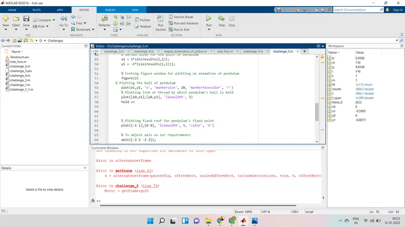
- Create a movie animation.
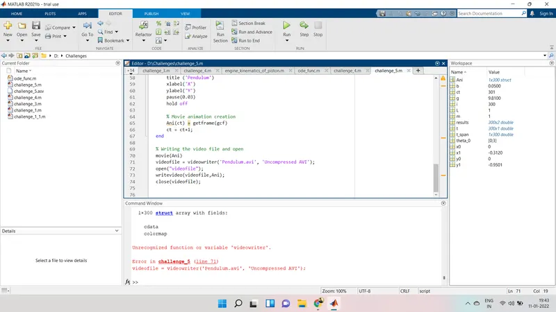
ERRORS SOLVING
- The errors faced are rectified and re-written, the main cause of error is miswritten of plotting and animation.
RESULTS
- PLOT
Angular displacement and angular velocity aganist time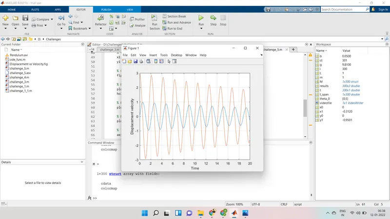
2. OUTPUT