Week 3 - Solving second order ODEs
Introduction
Solving pendulum problems using ODE45
Given Data
L=1 metre,
m=1 kg,
b=0.05.
g=9.81 m/s2.
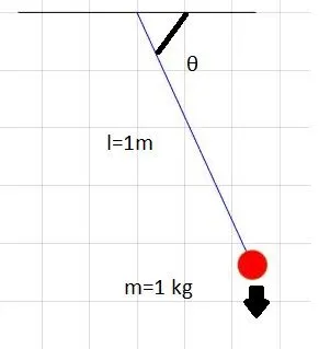
Solving
`b/m*(d theta_ 1)/dt+g/l*sin(theta)+(d theta_ 2)/dt = 0`
g = gravity in m/s2,
L = length of the pendulum in m,
m = mass of the ball in kg,
b=damping coefficient.
For solving splitting ODE as 1st order and 2nd order to solve equation
`(d theta_2)/dt=-b/m*(d theta_1)/dt-g/l*sin(theta)`
1st Order ODE
`theta2=(d theta_1)/dt`
`time, theta]=ode45((t,theta) function input parameter for solving`
which is velocity
2st Order ODE
`theta1=(d^2theta_1)/dt^2=d/dt(d theta_1)/dt^2=(d theta_2)/dt^2`
`[time, theta]=ode45((t,theta) function input parameter for solving`
for better understanding
from base equation
`b/m*(d theta)/dt+g/l*sintheta+(d^ 2 theta)/dt^2 = 0`
converting according to function & ODE to solve
`b/m*(d theta_1)/dt+g/l*sintheta_1+(d^ 2 theta_1)/dt^2 = 0`
`b/m*( theta_2)+g/l*sintheta_1+(d theta_2)/dt = 0`
`(d theta_1)/dt =theta_2`
`(d theta_2)/dt = -b/m*( theta_2)+g/l*sintheta_1`
ODE
ODE 45
Solve nonstiff differential equations — medium order method
ode45 is a versatile ODE solver and is the first solver you should try for most problems. However, if the problem is stiff or requires high accuracy, then there are other ODE solvers that might be better suited to the problem.
[t, result]=ode45(@(t,theta) p_funct (b,m,l,g,theta,t),tspan,theta0) also uses the integration settings defined by t, theta which is an argument created using the ode set function.
MATLAB CODE
Function
function dtheta_dt = p_funct (b,m,l,g,theta,t)
% P_FUNCT % creating function for an equation to solve ODE
% angular displacement
theta1=theta(1)

% angular velocity
theta2=theta(2)
% 1st order ode
dtheta1_dt=theta2
% secound order ode
dtheta2_dt=-b/m*theta2-g/l*sin(theta1)
% output rsult in single matrix
dtheta_dt=[dtheta1_dt; dtheta2_dt]
end
Main CODE
clear all
close all
clc

% given data
b=0.05
g=9.81
l=1
m=1

% angular displacement, angular velocity
theta0=[0;3];

% time spane
tspan=linspace(0,20,500);

%creating ODE
[t, result]=ode45(@(t,theta) p_funct (b,m,l,g,theta,t),tspan,theta0)

%Plotting
% time vs angular displacement
figure(1)
plot(t,result(:,1),'Color','r')
hold on
% time vs angular velocity
plot(t,result(:,2),'color','b')
hold off
xlabel('time')
ylabel('position')
legend('velocity','acceleration')
title('Analysis of pendulam')
grid on

figure(2)
plot(result(:,1),result(:,2),'color','r')
xlabel('velocity')
ylabel('acceleration')
title('Acceleration Vs velocity of pendulam ')

grid on
%animation
ct=1
for i=1:length(result(:,1))
    %creating position
    x0=0;
    y0=0;
    x1=-l*sin(result(i,1));
    y1=-1*cos(result(i,1));

    figure(3)
    %hold base
    plot([-0.5 0.5],[0 0],'color','k')
    hold on

    % pendulam strig
    line ([x0 x1],[y0 y1],'color','b')
    hold on

    % mass bob
    plot(x1,y1,'-o','MarkerSize',20,'MarkerFaceColor','r')
    grid on
    title('output movement of pendulam')
    axis([-1 1 -1.2 0.1])
    pause(0.001)
    hold off
    M(ct)=getframe(gcf)
    ct=ct+1

end

% save & create movie
% creating movie
movie(M)
% saving file
videofile = VideoWriter('pendulum.avi','Uncompressed AVI');
% opening file
open(videofile)
% writting file
writeVideo(videofile,M)
% closing file
close(videofile)
Plot
Position vs time with function changes
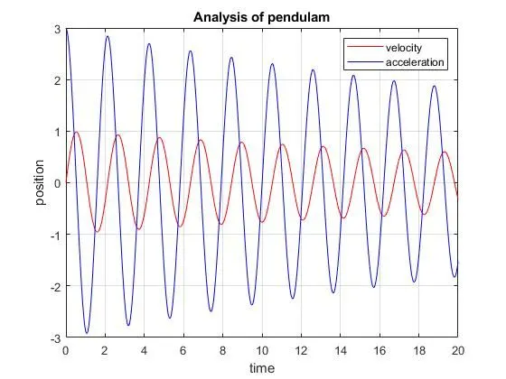
acceleration and velocity of the pendulum with respect to time and position
Acceleration Vs velocity variation function of time
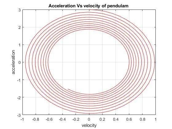
define 2nd order ODE VS 1st order ODE
Diagram output
Creation of line for base hold
creation of string
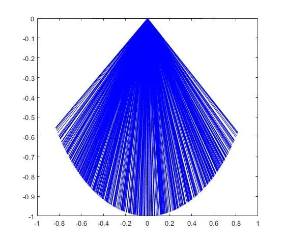
creation of bob
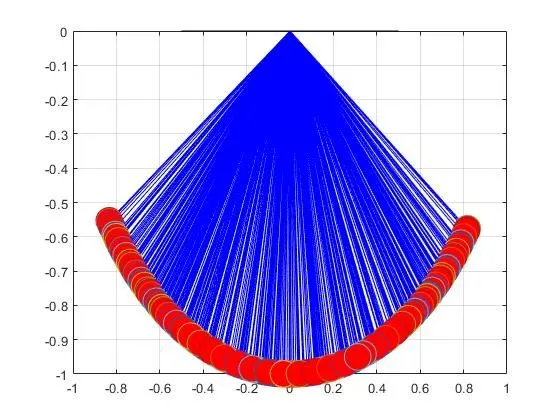
Error faced while
Error 1
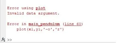
Error 2
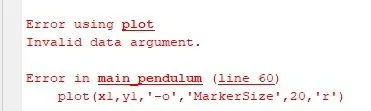
while creating diagram only bob without marker size & marker face colour shows error
output
video out
Conclusion
output for the pendulum is drawn using given data and ODE45 stiff function solved using Matlab
and video output is created for various time step
The output of ODE velocity & acceleration ploted graphically output