Week 3 - Solving second order ODEs

AIM: Write a program that will simulate the pendulum motion by using

the given conditions

L=1 metre,
m=1 kg,
b=0.05 N-s/rad-m,
g=9.81 m/s2,
Simulating the motion between 0-20 sec
Taking initial conditions as at t=0 , angular velocity=3 rad/sec and angular displacement =0

Objectve of this Programming

• To learn how to solve an Ordinary Differential Equation (ODE) using MATLAB.
• To solve ODE of a simple pendulum that represents its equation of motion.
• Understand the importance behind motion study of a simple pendulum
  

Main Programme of Matlab

Step wise Annotate,

clear all
close all
clc

%% Input Data
b = 0.05;  % Damping Coefficent
g = 9.81;  % Acceleration due to Gravity [m/s^2]
L = 1;     % Length of the Pendulum [m]
m = 1;     % Mass of the ball [kg]

%% Initial condition
theta_0 = [0;3];

%% Time Period of the motion of pendulum
t_span = linspace(0,20,500);

%% Solving ODE using ode45 
[t, results] = ode45(@(t,theta) ode_func_pendulum(t,theta,b,g,L,m), t_span, theta_0);

%% Result Plot

figure(1)
plot(t,results(:,1)) 
hold on
plot(t,results(:,2))
ylabel('Theta')
xlabel('Time')
title('Plot between Theta and Time')
legend('angular displacement','angular velocity'); 
hold off
grid on

%% For loop for animation of Simple Pendulum
theta = results(:,1);
ct=1;   % Intialization of counter
for i = 1:length(theta)
x = theta(i);

% Co-ordinate of Simple Pendulum
x0 = 0;
y0 = 0;
y1 = -L.*cos(x);
x1 = L*sin(x);

% Plot of Simple Pendulum
figure(2)
plot([x0 x1],[y0 y1],'linewidth',3,'color', 'b');
hold on
plot([1 -1],[0 0],'color','b');
plot(x1,y1,'marker','o','markersize',30,'color','r','MarkerFaceColor','g') %Ball plot
axis([-1 1 -1.5 1]);
hold off
grid on

pause(0.003)
M(ct)=getframe(gcf);
ct=ct+1;
end

% Creating Animation Video
movie(M)
videofile = VideoWriter('simple_pendulum.avi','Uncompressed AVI');
open(videofile)
writeVideo(videofile,M)
close(videofile)

Sub Function

ode_func_pendulum sub function is use inside the ode45 which is a buil-in function of Matlab Library for solving ODEs.

function [dtheta_dt] = ode_func_pendulum(t,theta,b,g,L,m)

% Initializing the value
theta_1 =theta(1);
theta_2 =theta(2);
dtheta_1_dt = theta_2;
dtheta_2_dt = -(b/m)*theta_2 -((g/L)*sin(theta_1));

% Resultant Matrix
dtheta_dt = [dtheta_1_dt; dtheta_2_dt];
end

Output Plot

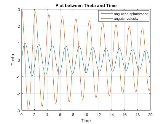
This Plot shows nature of Angular Dispalcement and Angular Velocity with respect to Time from initial Conditions where, Angular Dispacement = 0 and Angular Velocity = 3 rad/s where Time t=0.

Animation Result

The animation of a Simple Pendulum.

https://drive.google.com/drive/u/1/folders/1VhSBnKIzQWELbRC-_laq4mynfDV7adOS

Conclusion

I have understood how to solve a second ODEs using MATLAB with Buil-in Function.I have also achieve the study of the simple pendulum motion and its animation.

Error While Programming

1. Many typo error making programme errorneous.

2. I wrote sind,Cosd insted of writting Sin,Cos , make the animation slower, very small fluctuation and the video file also made larger file size like 300Mb neither its generally 15Mb to 25Mb.