Week 3 - Solving second order ODEs

AIM:- To solve 2nd order ODE and to give motion to pendulum with MATLAB.

Objective:-

To solve 2nd order ordinary differential equations and with that values giving motion to pendulum.

Introduction:-

A pendulum is a weight suspended from a pivot so that it can swing freely.[1] When a pendulum is displaced sideways from its resting, equilibrium position, it is subject to a restoring force due to gravity that will accelerate it back toward the equilibrium position. When released, the restoring force acting on the pendulum's mass causes it to oscillate about the equilibrium position, swinging back and forth. The time for one complete cycle, a left swing and a right swing, is called the period. The period depends on the length of the pendulum and also to a slight degree on the amplitude, the width of the pendulum's swing.

CODE EXPLANATION:-

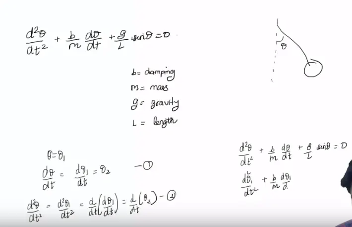
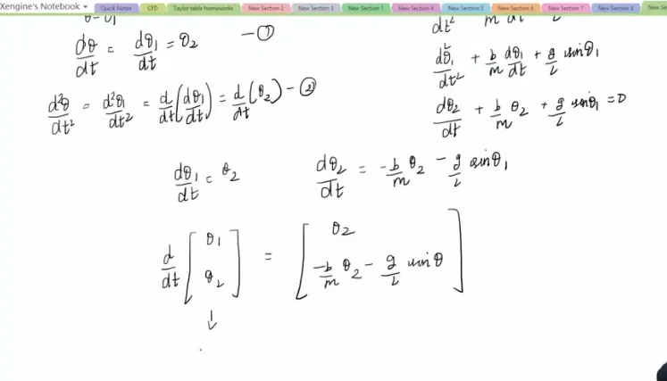
So first 2nd order ode is need to be converted into 1st order ode by assuming theta=theta1 likewise mention in abive pictures.

then define inputs as damping b, gravtity force g, length l and mass m. then define initial condition as theta. then define span of time.

for solve ode use ode45 command give necessary inputs and define them. then open new script.

in that script define ode equations like mentioned in the pictures. with he function command just give link to both the files.

for motion of pendulum define the points of fixed horizontal line then define the points of vertival line which will going to be change wrt time.

now at the end of that vertival line make circle with marker command. then use for loop for motion as metioned in the code.

plot all the define points in the loop ciommand. make animation.

MATLAB CODE:-

%To solve 2nd order ODE 

close all
clear all
clc

%Inputs
b=0.05;
g=9.81;
l=1;
m=0.1;

%Initial condition
theta_0=[0;5];

%Time points
t_span=linspace(0,10,500);

%Solve ODE
[t,results]=ode45(@(t,theta) ode_func(theta,b,g,l,m),t_span,theta_0);

% %Pendulum animation
% for i=1:length(t,results);
% end   
    

%Plotting
figure(1)
plot(t,results(:,1))
hold on
plot(t,results(:,2))
legend('Angular displacement','Angular velocity')

ct=1
for i=1:length(t)
    x=l*sin(results(i,1));
    y=-l*cos(results(i,1));
    
    figure(2)
    
    plot([-1,1],[0,0],'linewidth',5) %plotting fixed line
    hold on
    plot([0,x],[0,y],'linewidth',5) %plotting pend 
    plot(x,y,'Marker','o','MarkerSize',20,'MarkerFacecolor','g','Markeredgecolor','k') %plotting bob
    axis([-2 2 -2 2])
    pause(0.01);
    M(ct)=getframe(gcf);
    ct=ct+1;
    hold off
end

 movie(M);
    videofile=VideoWriter('pendulum.avi','uncompressed AVI');
    open(videofile);
    writeVideo(videofile,M);
    close(videofile)

function [dtheta_dt]=ode_func(theta,b,g,l,m)

theta1=theta(1);
theta2=theta(2);
dtheta1_dt=theta2;
dtheta2_dt=-(b/m)*theta2-(g/l)*sin(theta1);
dtheta_dt=[dtheta1_dt;dtheta2_dt];
end

RESULTS:-

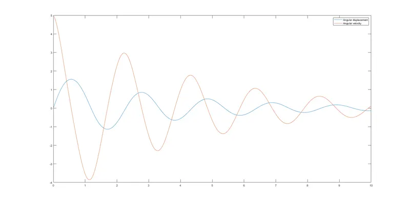
VIDEO= https://drive.google.com/file/d/1zLsgjhDxgQ2HAjlR2uqkeM-3dLFUa2eH/view?usp=sharing