Week 3 - Solving second order ODEs

AIM OF THE PROJECT:

To write a program to solve an Ordinary Differential Equation (ODE) which represents the equation of motion of a simple pendulum with damping.

THEORY:

What is ODE:

In mathematics, an ordinary differential equation (ODE) is a differential equation containing one or more functions of one independent variable and the derivatives of those functions. The term ordinary is used in contrast with the term partial differential equation which may be with respect to more than one independent variable.

In Engineering, ODE is used to describe the transient behavior of a system. A simple example is a pendulum

The way the pendulum moves depends on Newton's second law. When this law is written down, we get a second order Ordinary Differential Equation that describes the position of the "ball" with respect to time.

Similarly, there are hundreds of ODEs that describe key phenomena and if you have the ability to solve these equations then you will be able to simulate any of these systems.

What is a simple pendulum:

A pendulum is a body suspended from a fixed support so that it swings freely back and forth under the influence of gravity. When a pendulum is displaced sideways from its resting, equilibrium position, it is subject to a restoring force due to gravity that will accelerate it back toward the equilibrium position. When released, the restoring force acting on the pendulum's mass causes it to oscillate about the equilibrium position, swinging it back and forth.

figure: Simple Pendulum

The differential equation which represents the motion of a simple pendulum is

.........................

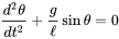
Eq. 1

where

g is the acceleration due to gravity,

l is the length of the pendulum, and

θ is the angular displacement.

Governing Equation:

Ordinary Differential Equation (ODE) representing equation of motion of a simple pendulum with damping –

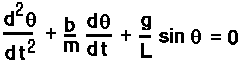.......................Eq. 2

where,

g = gravitational acceleration (m/s²)

L = length of the pendulum (m)

m = mass of the ball (kg)

b = damping coefficient

Input Values we are taking in this project are:

L=1 meter,

m=1 kg,

b=0.05.

g=9.81 m/s2.

Simulating the motion between 0-20 sec, for angular displacement=0,angular velocity=3 rad/sec at time t=0.

Function Program:

%program to make a function to solve 2nd order ODE of a simple pendulum

function[dtheta_dt] = ode_func(t,theta,b,g,l,m)
theta1 = theta(1)
theta2 = theta(2)
dtheta1_dt = theta2;
dtheta2_dt = -(b/m)*theta2-(g/l)*sin(theta1);
dtheta_dt = [dtheta1_dt;dtheta2_dt];
end

Explanation: In this program, we are creating a function by deriving the governing equation named "ode_func(t, theta, b, g, l, m)" to be called in the main program with input parameters t, theta, b, g, L and m.

Main Program:

% program to find solve a 2nd order ODE of a simple pendulum 
% and animate the motion of a simple pendulum

%inputs
%given parameters
b = 0.05; % damping coefficient
g = 9.81; % gravitational acceleration
l = 1;    % Length of the pandulum
m = 0.1;  % mass of the ball

% Initial condintions of Displacement and Velocity
theta_0 = [0;3];

% time points distributed over an array
t_span = linspace(0,20,500);

% soloving the ODE using inbuilt ODE solver 'ode45'
[t,results] = ode45(@(t,theta) ode_func(t,theta,b,g,l,m),t_span,theta_0);

% Plotting curves between displacement and velocity vs time
figure(1)
plot(t,results (:,1)) % displacement v/s Time
hold on
plot(t,results (:,2)) % velocity v/s Time
grid on
title('Transient Behaviour')
xlabel('Time')
ylabel('Plot (Displacement & Velocity)')
legend('Displacement','Velocity')


% Making the animation video of a simple pendulum motion
figure(2)
ct = 1;
for i = 1:length(t_span)
    RESULTS = results(i);
    
    % Coordinates of start point
    x0 = 0;
    y0 = 0;
    
    % Coordinates of end point
    x1 = l*sind(RESULTS);
    y1 = -l*cosd(RESULTS);
    
    % Plotting
    % Plot representing the massless thread
    plot([x0 x1],[y0 y1],'linewidth',2,'color','g');
    hold on
    
    % Plot representing ceiling from which the pendulum hangs
    plot([-0.5 0.5], [0 0],'linewidth',5,'color','b');
    
    % Plot representing the bob
    plot(x1,y1,'marker','o','markersize',15,'markerfacecolor','r');
    
    title('SIMPLE PENDULUM MOTION')
    axis([-1.5 1.5 -1.5 0.5]);
    pause(0.00005);
    
    % Hiding the axes of the plot
    set(gca,'XTick',[], 'YTick', [])
    
    M(ct) = getframe(gcf);
    hold off
    ct=ct+1;
end
 
% Animating the motion of simple pendulum
movie(M)
videofile = VideoWriter('simple_pendulum.avi','Uncompressed AVI');
open(videofile)
writeVideo(videofile,M)
close(videofile)

Explanation:

1. The given values are specified and the initial condition is imposed.
2. Timespan over which the pendulum’s transient behavior has to be observed is also defined.
3. Now, the inbuilt ODE solver is used to calculate the results along with the ode function that we made with some input parameters for the governing equation.
4. Further, we plot the Displacement v/s Time and Velocity v/s Time graphs on the same figure to study the respective behaviors.
5. After the plotting, for making the animation of the pendulum motion we make a simple pendulum figure using three plot commands under for loop in the same plot representing the massless bar, ceiling, and the pendulum bob, and the movie is done using Movie Command and movie file is saved by using VideoWriter function.

OUTPUT:

The plot of the Transient Behaviour of Displacement and velocity w.r.t. Time:

Link for the animation movie:

https://youtu.be/rAcjIkfXtZc

Errors Occurred:

Conclusion:

From the above outputs, we can clearly see the transient behavior of displacement and velocity of a simple pendulum having a damping system with respect to time and we can clearly visualize the system in the animation video of the simple pendulum.

References:

https://en.wikipedia.org

https://services.math.duke.edu