Week 3 - Solving second order ODEs

Aim:

To Simulate Simple Pendulum by solving ODE

Governing Equations:

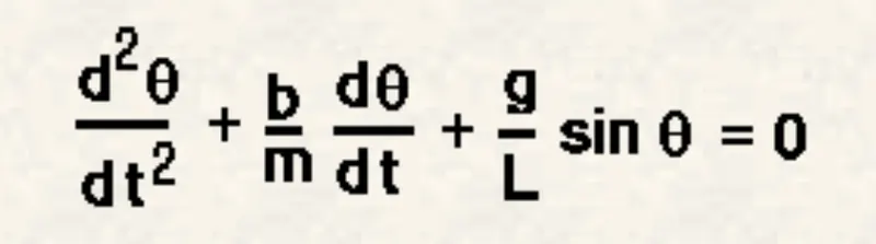
Here b is the damping coefficient,

L = length of the string,

m = mass of the bob,

g = gravitational pull

On solving the above equation, we get angular velocity w.r.t. time

Objective:

To simulate Python code to solve higher order ODE and obtain animation for movement of a simple pendulum.

Code:

#Python code to solve second order ODE and create animation of a Simple pendulum with solutions obtained from ODE

import math
import matplotlib.pyplot as plt
import numpy as np
from scipy.integrate import odeint
#Import modules required to use mathematical values like pi, numpy for using linspace, odeint to solve ODE

#Function to calculate values of theta angle for angular displacement and angular velocity
def model(theta,t,b,g,l,m):
	theta1 = theta[0] #Theta1 will carry value of displacement
	theta2 = theta[1] #Theta2 will carry value of velocity
	dtheta1_dt = theta2
	dtheta2_dt = -((b/m)*theta2)-((g/l)*math.sin(theta1)) #Formula to calculate angle for damped osciallation w.r.t. time
	dtheta = [dtheta1_dt,dtheta2_dt]
	return dtheta #After calculating the value of theta it would be returned when function would be called

#Parameters for Pendulum
b=0.1 #Damping coefficient
l =1 #metre, length of string
m =1 #Kg, mass of bob
g= 9.81 #m/s^2 Gravitational pull 

#Initial Condition 
#Here 1st row in theta_int represents initial displacement which is 0 metre and initial angular velocity is 3 rad/sec 
theta_int = [0,3]
#Counter variable to asssign image no to save png files
ct=1

#Total time for motion is 20 seconds so extracting 300 values in between 0 and 20 seconds
time = np.linspace(0,20,300)

#Solving ODE
theta = odeint(model,theta_int,time,args=(b,g,l,m))
#odeint takes in the parameters for the function model and timespan to integrate the values
#Theta will carry two different columns, 1st column for displacement and 2nd column for velocity

#With help of a for loop elements of displacement from theta
for th in theta[:,0]:
	"""
	In a pendulum at left or right position would create a triangle, so on breaking the components
	xx represents the horizontal position of the pendulum
	yy represents the vertical position of the pendulum
	"""
	xx = l*math.sin(th)
	yy = -l*math.cos(th)
	plt.figure()
	plt.plot([-0.5,0.5],[0,0])
	plt.plot([0,xx],[0,yy])
	plt.plot(xx,yy,marker='.',markersize=60)
	plt.xlim([-1.2,1.2])
	plt.ylim([-1.2,0.2])
	plt.xlabel('Displacement')
	#Every plot would be saved in a new figure and would be saved in a sequential order
	plt.savefig('%04d.png'%ct)
	ct=ct+1

Conclusion:

The Python code has been designed such that the values for damping, length and mass could be changed to alter results. Also, the time span could be increased or decreased depending on the oscillation animation required.