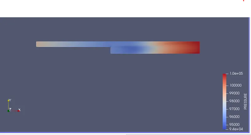
Week 3: Flow over a backward facing step
Aim
1) To simulate the backward step flow for three different mesh grid sizes by using convergent science and paraview.
2) To show various velocity and pressure contours for the different mesh size.
3) to show the various plots for velocity, pressure, mass flow rate and cell count for different mesh sizes.
4) to study the turbulent flow cherectoristics in backwar flow step.
Introduction
Backward-Facing Step (BSF) flow is one representative model for separation flows, which can be widely seen in aerodynamic flows (airfoil, spoiler, high attack angle process), engine flows, condensers, vehicles (cars, boat), heat transfer systems, and even the flow around buildings, etc. The flow separation after a simple stage will introduce separation bubble formation, evolution and re-attachment process, which is dependent on the BFS geometric design, the inlet and outlet conditions, turbulent intensity, as well as heat transfer conditions. In the past decades, it has been widely studied by various theoretical, experimental and numerical methods. Considering the importance of BFS flow in both theoretical and engineering aspects. It is shown that the step size (duct expansion ratio) will define the basic re-circulation and re-attachment process.
it is basic model involving the important features of flow seperation, vortex generation, a free share flow seperation and reatachment. A backward flow includes an inflow of uniform velocity laminer or turbulent from a channel to a step on either side with a step of height h.
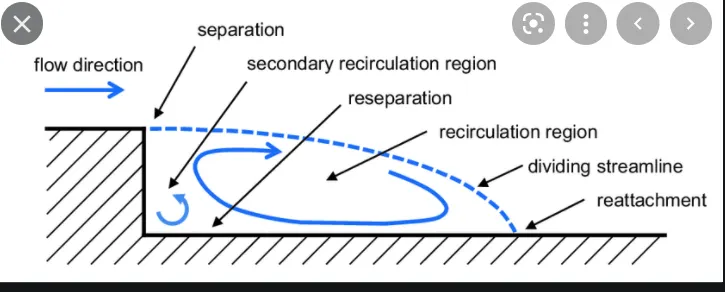
The flow fluid is divided into four regions namely seperated shear layer, the recerculation region under the shear layer, the reattachment region and the recovered boundry layer.
Flow with seperation and reattachment has been a subject of fundamental fluid dynamics research. The pressence of seperated flow together with the reattaching flow give rise to incleased unsteadiness, pressure fluctuations, structure viberations and noise. It also exhibits an unsteady structure with a large scale vortox in seperated shear layer and low frequency motion around the reattachment region with fluctuation af an instantaneous reattachment point.
Aflow is termed as turbulent when the inertial forces are greator then viscous forces of fluid, resulying in choatic fluctuations. Turbulent flow occurs in veriety of industrial problems. Turbulent flow over a backward facing step is one of the classical tests to validate turbulence models in CFD. In the present work steady state turbulent flow over a backward facing step was simulated using converge with Renormalization group (RNG) `k-epsilon`model to account the turbulence viscosity.
Different regions are shown in the figure below
Base Grid taken for three cases are given in table below
| Base grid | dx | dy | dz |
| case1 | 0.002m | 0.002m | 0.002m |
| case2 | 0.0015m | 0.0015m | 0.0015m |
| case3 | 0.001m | 0.001m | 0.001m |
Time taken is given bellow
| Base grid | No. of processors used for simulation | Time taken |
| case1 | 4 | 190.69sec |
| case2 | 4 | 119.16sec |
| case3 | 4 | 309.004sec |
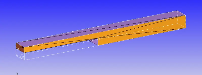
3D view of geometry
Velocity, pressure, cell count and mass flow rate at inlet and out let for all cases are shown below
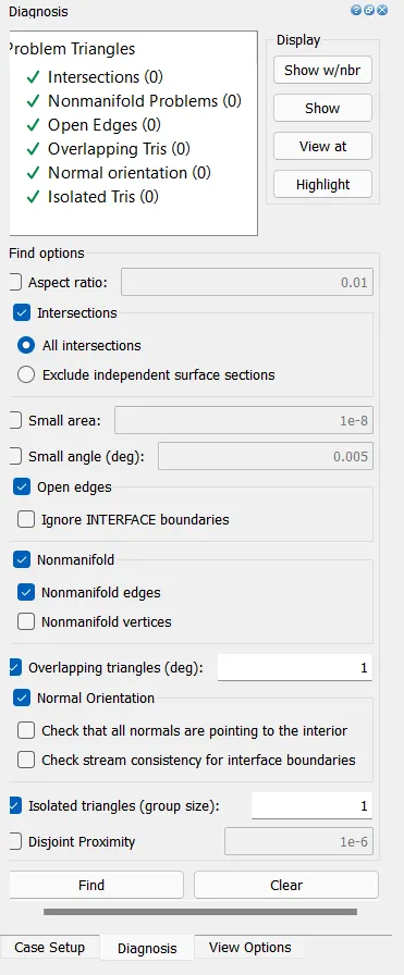
Diagnosis
CASE SETUP
- Application Type: Time based
- The Flow is general flow which contain air as a material.
- Air contain species of mixture o2 and N2 which will flow through the required geometry.
- Global transport parameters, the prandle number is 0.9 and Schmidt number is 0.78
Simulation Parameters
Run Parameters
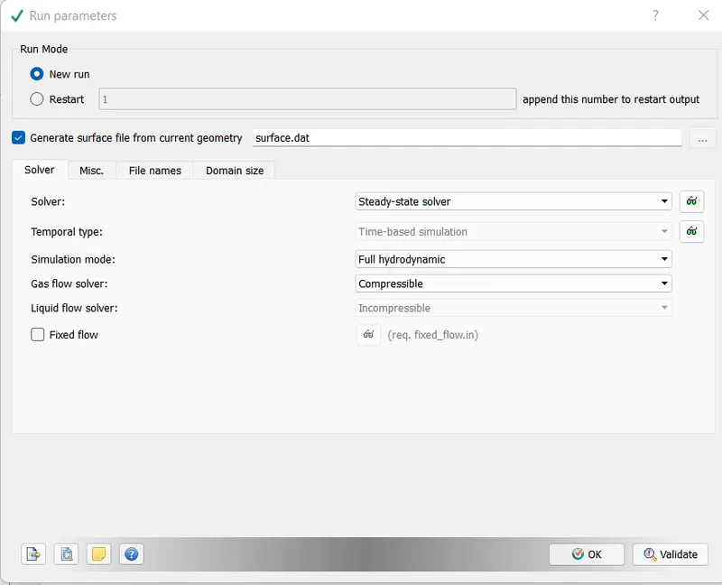
Simulation Time Parameter
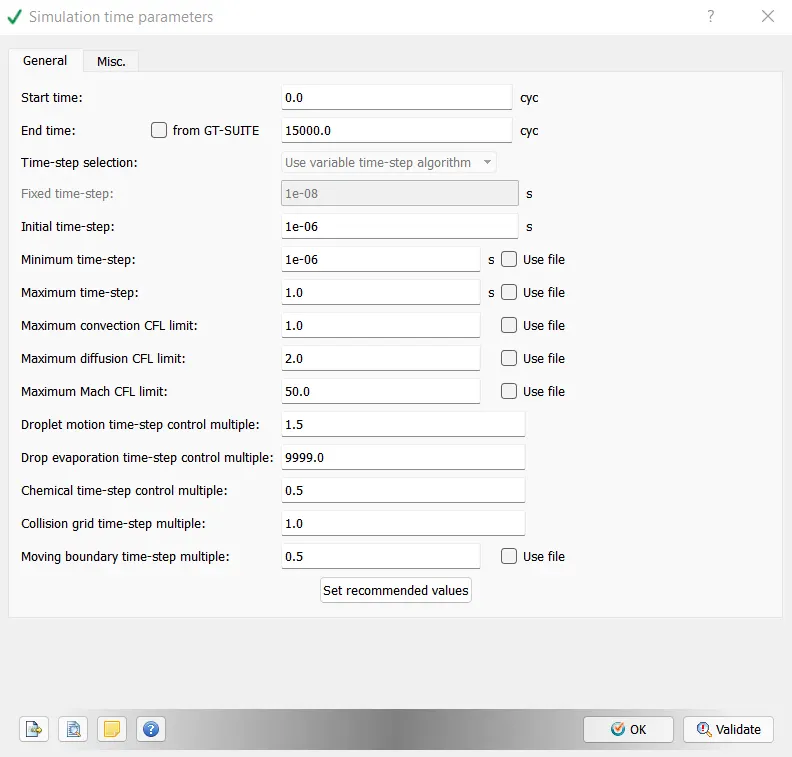
Solver Parameter
- The Navier Stroke equation should be pressure based solver and take remaining as default values.
Steady State Monitor
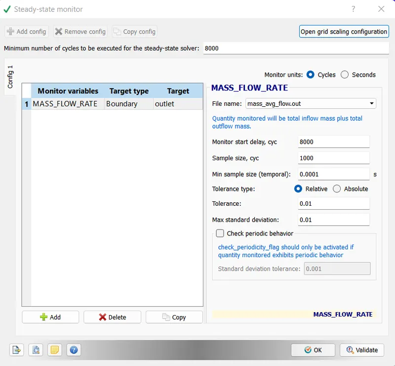
Initialization and Boundry Conditions
Inlet
- Pressure at inlet is 1.5e5
- temperature should be 300K
- boundry type: In flow
Outlet
- Pressure: 1e5
- temperature: 300k
- Boundary type: out flow
Top and Bottom
- Boundary: wall
- Boundary condition: Law of wall
- Temperature 300K
Front 2D
- Boundry : 2D
Back 2D
- Boundary: 2D
Physical Models
- In physical models enable tubulance modeling and solver should be selected as RNG `k -epsilon` and put remaining values as default.
Grid Control
- In grid control enable fixed embedding and base grid.
- Enter grid values and go to fixed embedding
- add entity type: boundary
- Boundry id: Top and bottom
- Mode: Permanent
- Scale: 1
- Embedded Layers: 1
- after entering all values click ok
Output and Post Processing
- Post variables selection and output files are default values.
- In output files we have to give time intervale to write the output data = 150 cycles. It means the output of simulation files will be stored after 150 cycles.
RESULTS
Case 1 (mesh size 0.002m)
pressure at inlet
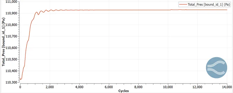
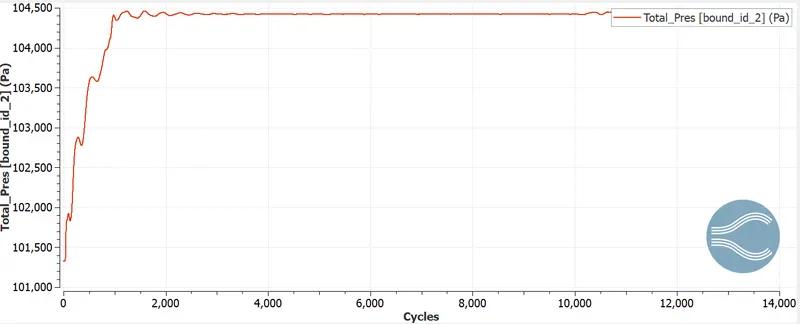
pressure at out let
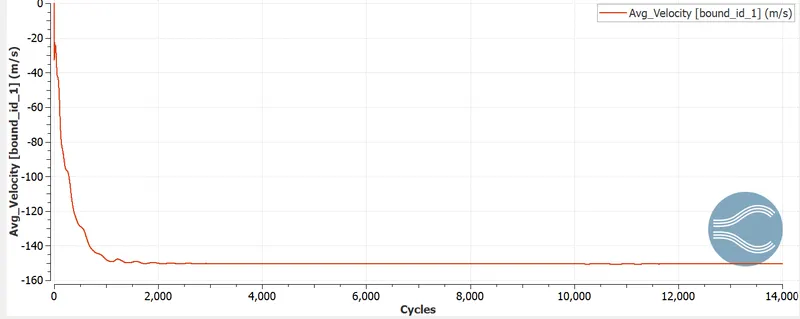
Average velocity at inlet
Average veoocity at out let
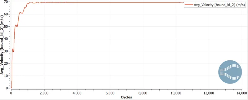
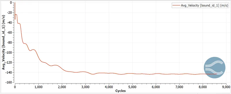
Inlet velocity approches the value of -140m/s, Where as outlet velocity takes a value of 70m/s. The opposite sign gives a clear indication that the momentum has been conserved. There is a difference in value oif velocity as the area of cross section increases as the air flows from left to right.
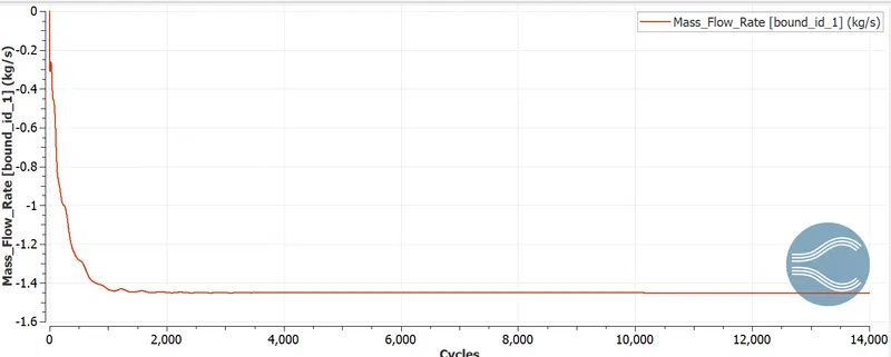
mass flow rate at inlet
mass flow rate at out let
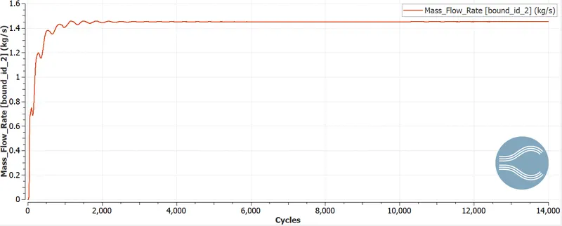
As air enters the domain there is a mass flow rate of 1.4 Kg/s. When air enters there is a negitive sign because the direction of flow is opposite to the norma. The opposite sign cancell each other to say that mass is conserved.
Total Cell count for case 1
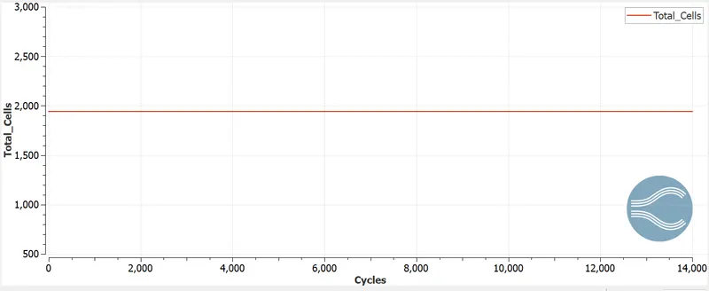
Total cell count for case 1 is almost 1999 cells
Case 2 (mesh size 0.0015m)
Average velocity at inlet
Average velocity at outlet
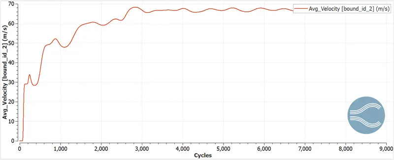
Inlet velocity approches the value of -140m/s, Where as outlet velocity takes a value of 70m/s. The opposite sign gives a clear indication that the momentum has been conserved. There is a difference in value oif velocity as the area of cross section increases as the air flows from left to right.
Pressure at inlet
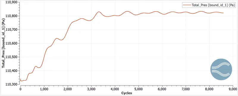
Pressure at outlet
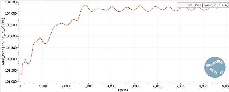
Mass flow rate at inlet
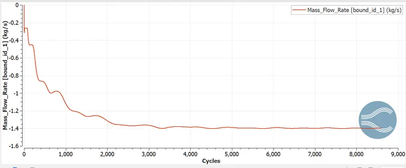
Mass flow rate at outlet
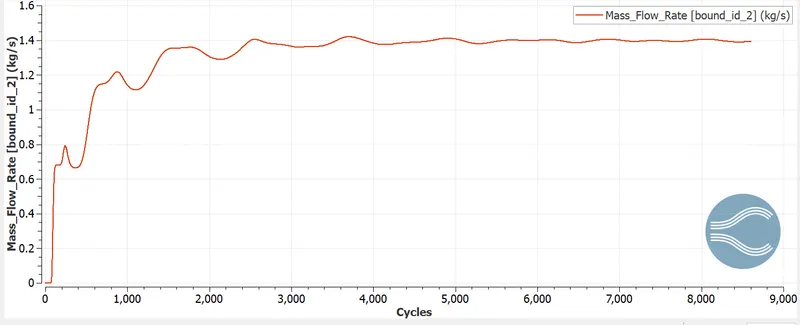
As air enters the domain there is a mass flow rate of 1.4 Kg/s. When air enters there is a negitive sign because the direction of flow is opposite to the norma. The opposite sign cancell each other to say that mass is conserved.
Total cell count for mesh size 0.0015m
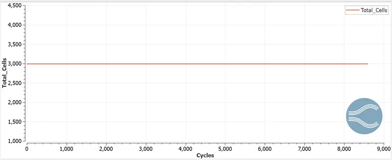
Total cell count for case 1 is almost 3000 cells
Case 3(mesh size 0.001m)
Average velocity at inlet
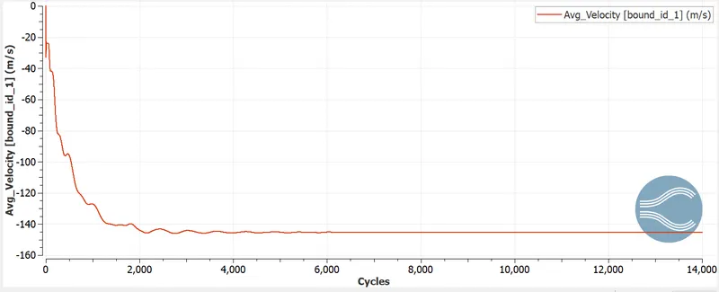
Average velocity at outlet
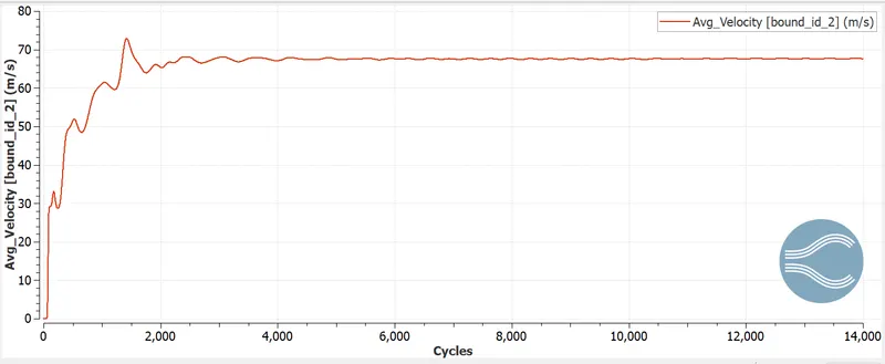
Inlet velocity approches the value of -140m/s, Where as outlet velocity takes a value of 70m/s. The opposite sign gives a clear indication that the momentum has been conserved. There is a difference in value oif velocity as the area of cross section increases as the air flows from left to right.
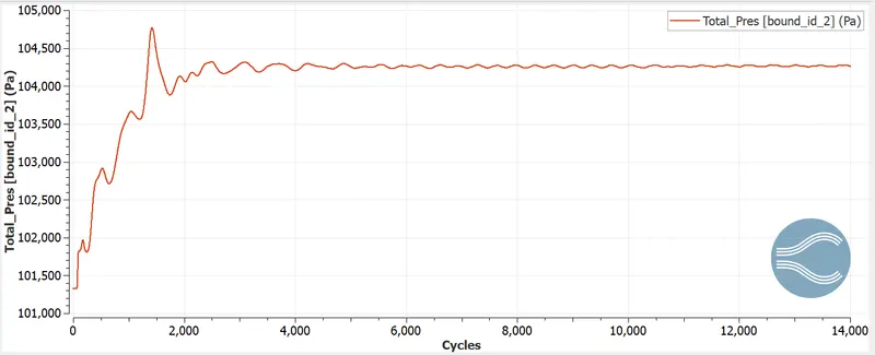
Total Pressure at inlet
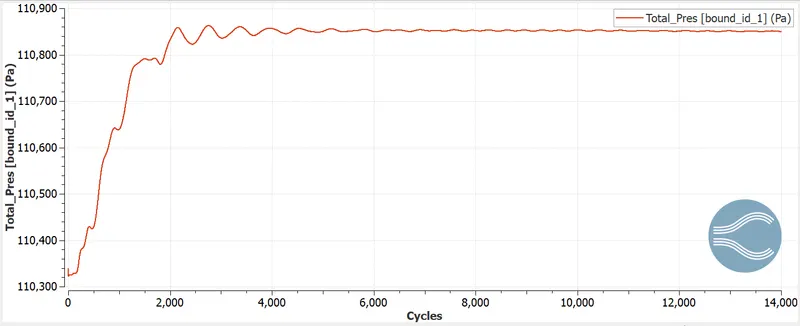
Total pressure at outlet
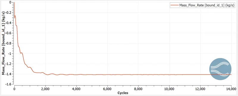
Mass flow rate at inlet
Mass flow rate at outlet
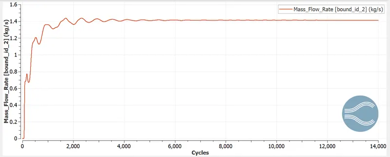
As air enters the domain there is a mass flow rate of 1.4 Kg/s. When air enters there is a negitive sign because the direction of flow is opposite to the norma. The opposite sign cancell each other to say that mass is conserved.
Total cell count
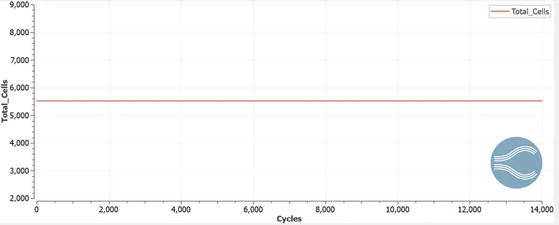
Total cell count for case 1 is almost 5500 cells
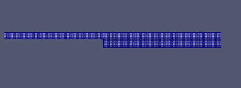
Mesh for case 1

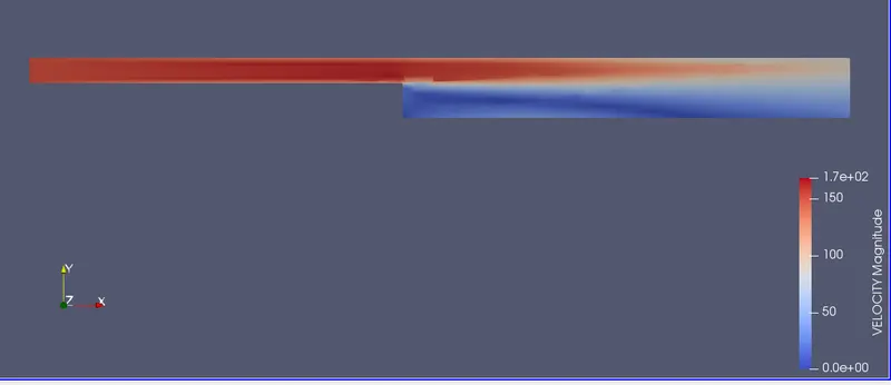
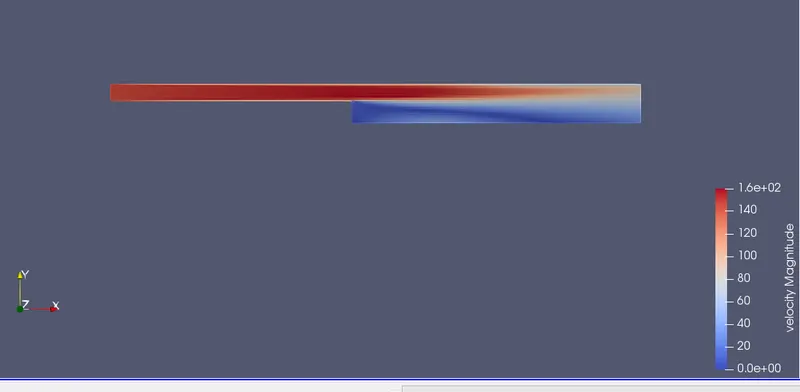
Velocity Contour for case 1
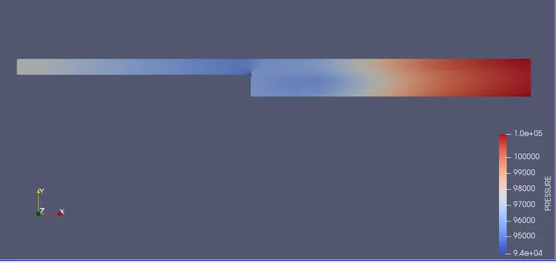
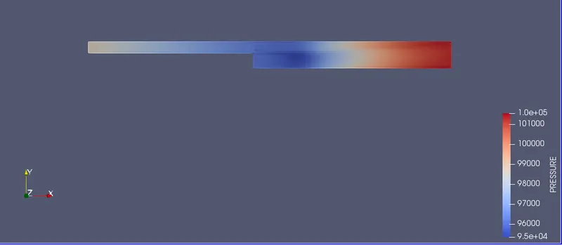
Pressure contour for case 1
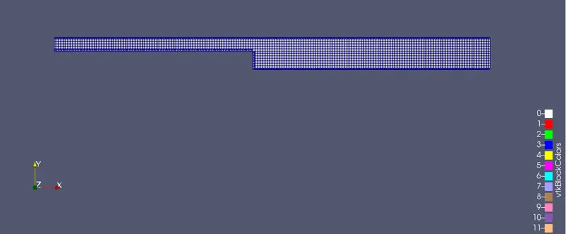
Mesh for case 2
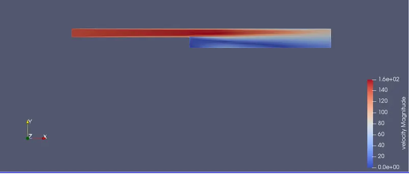
Velocity Contour for case 2
Pressure contour for case 2
Mesh for case 3
Velocity Contour for case 3
Pressure contour for case 3