Flow over a backward facing step

Introduction

Many engineering application such as aerodynamic flows, engine flows, condensers, vehicles, heat transfer systems, and flow around buildings etc. involves flow separation and reattachment.

Backward-Facing Step is a representative model for domenstrating separation flows. The flow separation after a simple stage introduces separation bubble formation, evolution and re-attachment process, which is dependent on the BFS geometric design, the inlet and outlet conditions, turbulent intensity, as well as heat transfer conditions.

Objective

The scope of present study is to simulate the backward facing step problem and observe the seperation and reattachment region using a CONVERGE CFD software. 

Also, the study covers the effect of results with varying grid size.

Outline

In order to achive the objective the study has been planned as below:

Case 1: The grid size has been set to 2e-3m

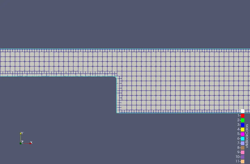
Case 2: The grid size has been set to 1.5e-3m

Case 3: The grid size has been set to 1e-3m

Simulation

Application type

The application type is choosen to be timee based.

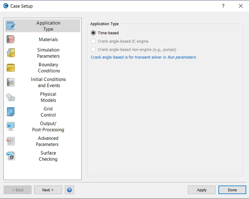
The geometry was imported from the given source and later it was modified for use in CONVERGE CFD.

Geometry

fig. The backward Facing Step Geometry

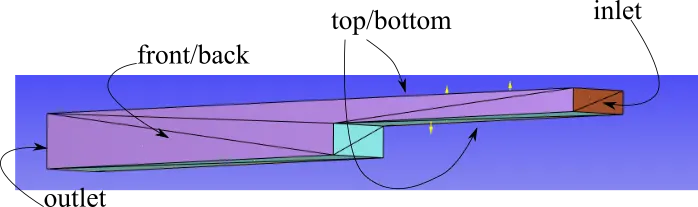
fig. The name of boundaries defined in the backward facing step

Materials

In the case setup, the material is choosen to be gas.

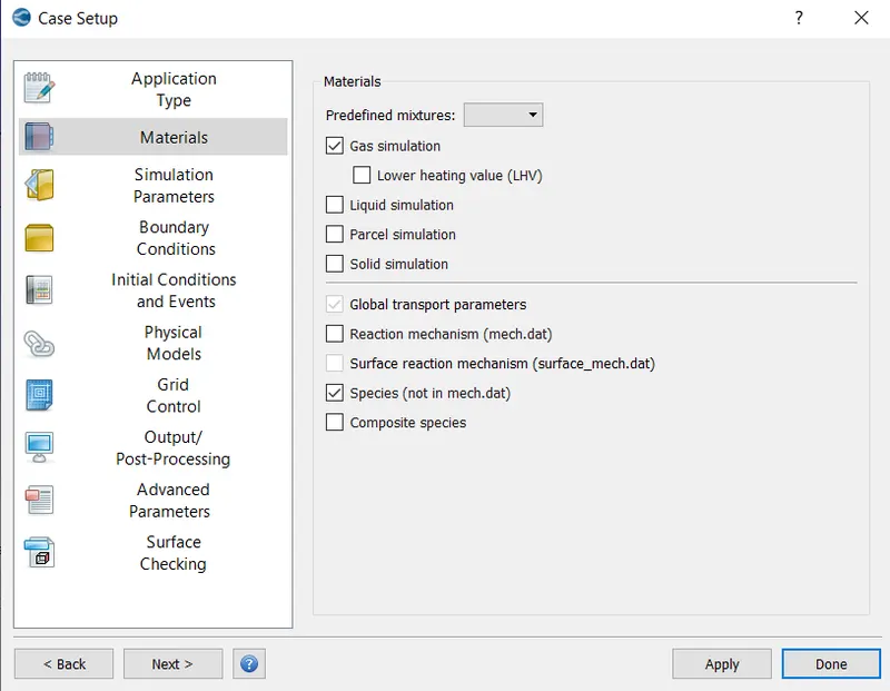
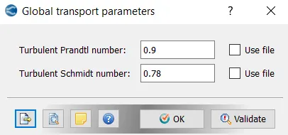
The gas transport properties are choosen as the default value

The equation of state and critical temperature as been left as default value.

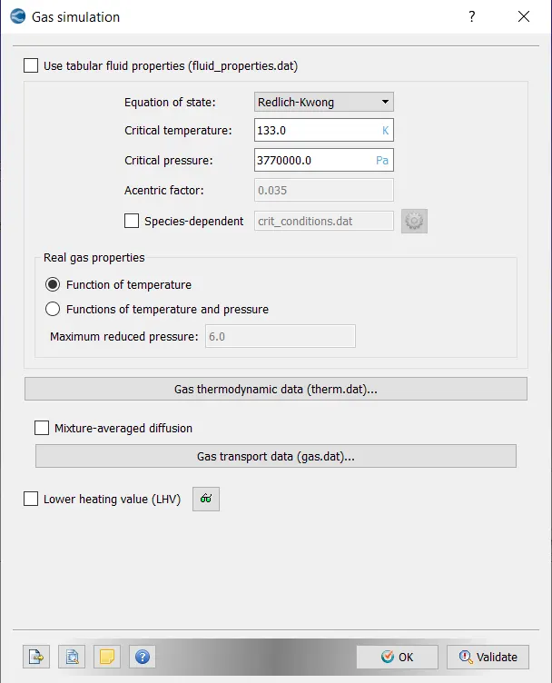
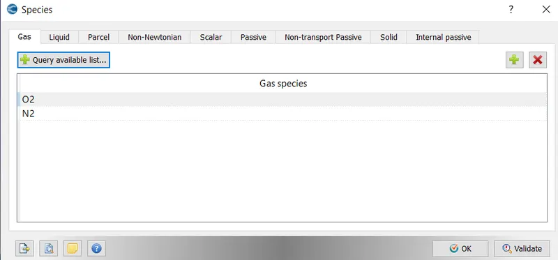
Since we are not dealing with any reaction in our simulation, the accuracy of species defition is not required, so only major components like oxygen and nitrogen is chosen.

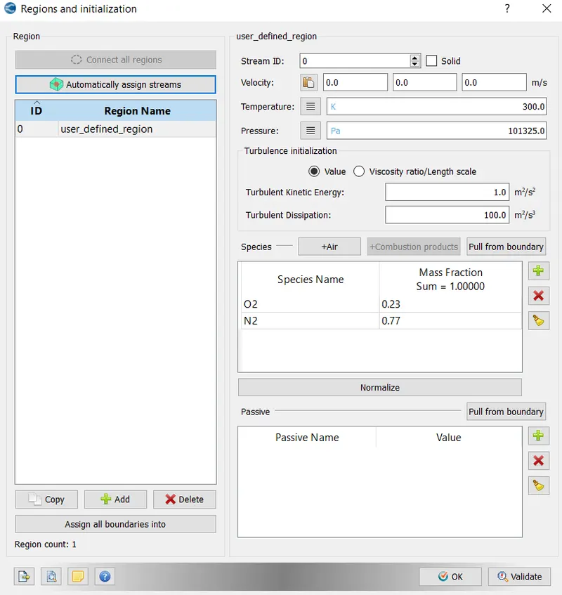
Regions and initial condition

The volume has been defined under one region called user_defined_region. The initial pressure is set as that to be equal to 101325 Pa.

Solver Parameters

The steady state solver has been chosen for the given problem as after some time the flow will be in steady state and it is of our main importance.

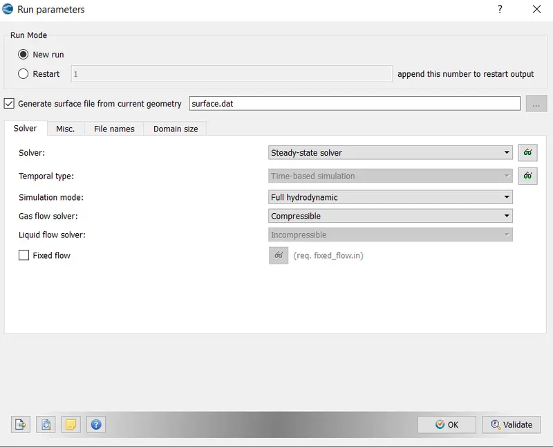
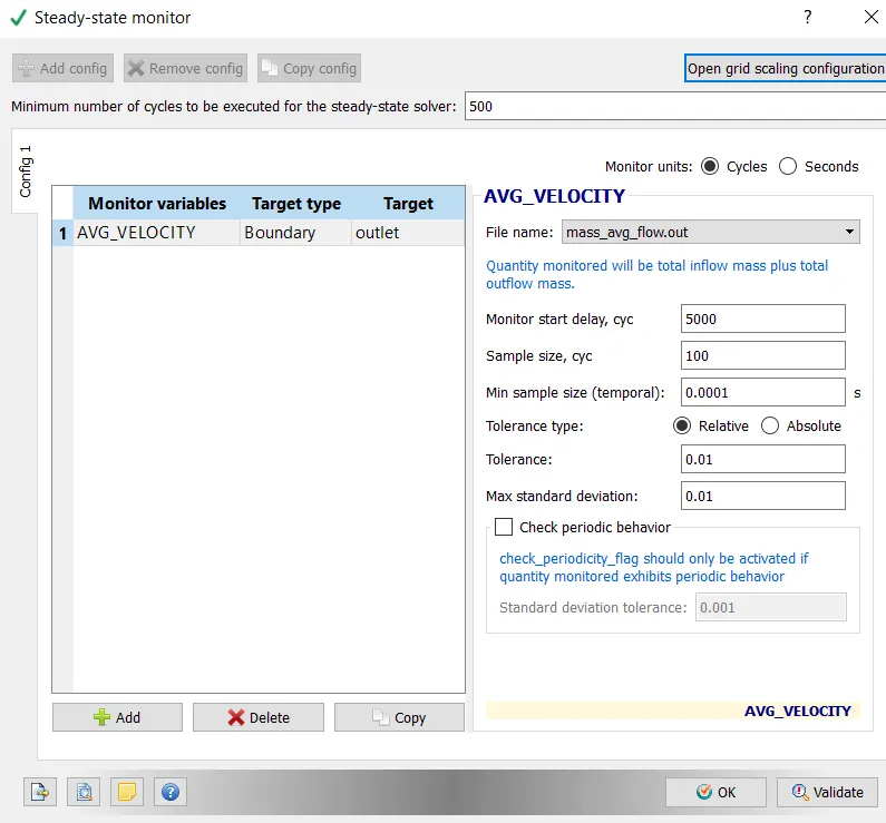
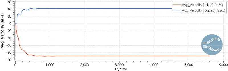
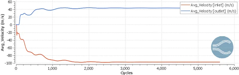
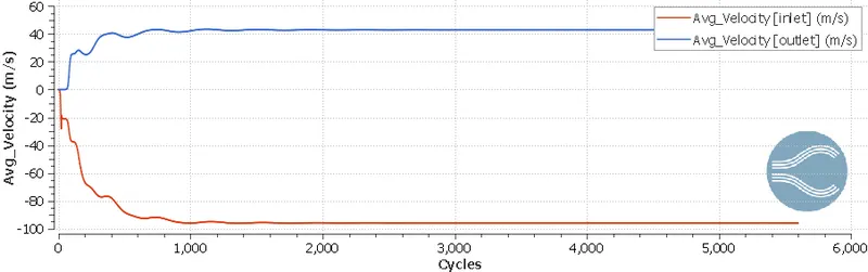
Average velocity has been defined as the monitoring variable. The convergence check will be initialted at 5000 iterations.

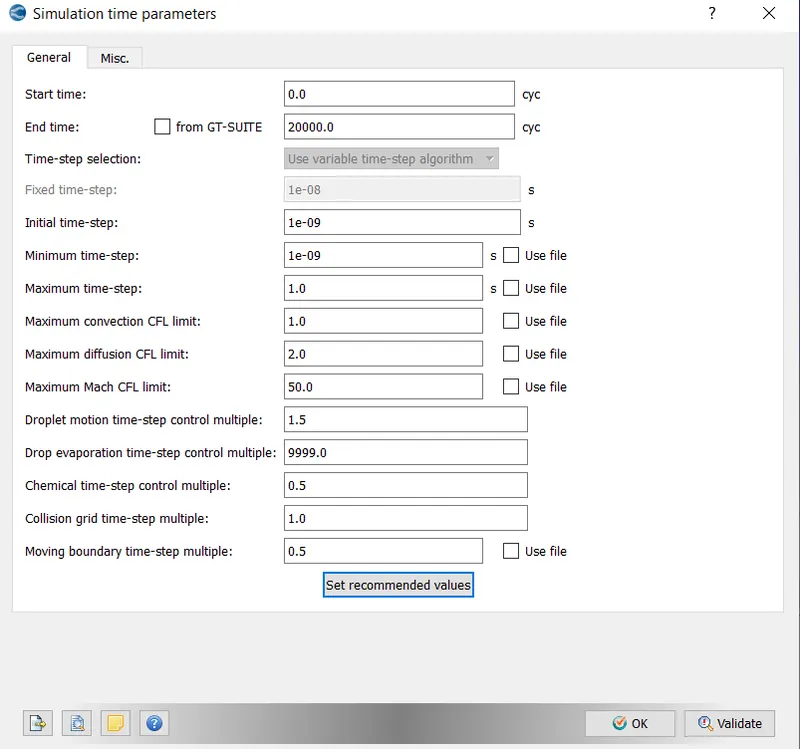
The maximum cycle for the simulation has been chosen to be 20,000. For automatic time step calculation and accurate results, the maximum convection cfl has been reduced to 1.

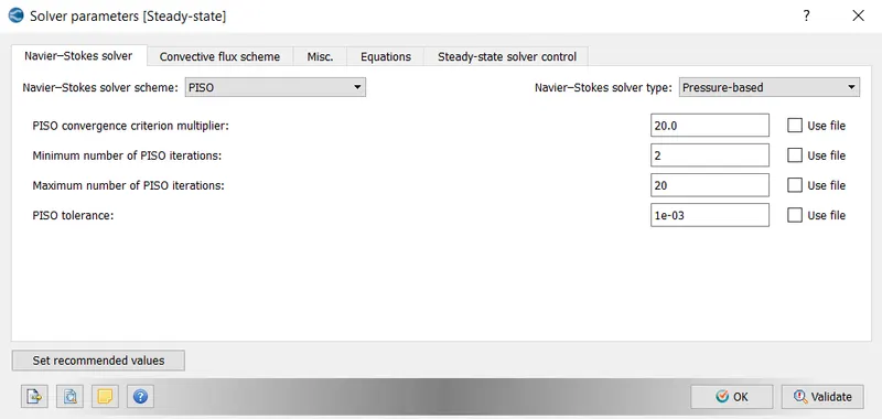
Pressure Based solver is choosen in the steady solver type.

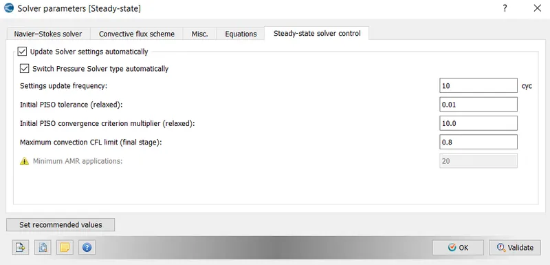
Maximum convection CFL limit of final stage is chosen to be 0.8.

Boundary Conditions

inlet

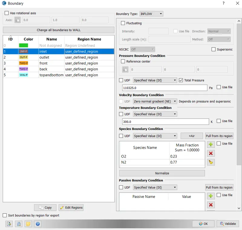
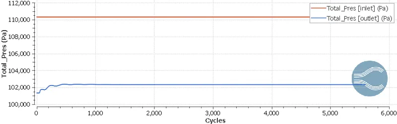
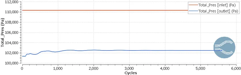
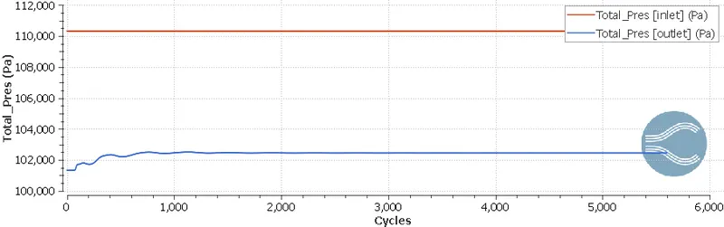
Inlet boundary has been given Inflow boundary type with a fixed total pressure of 110325 Pa.

Outlet

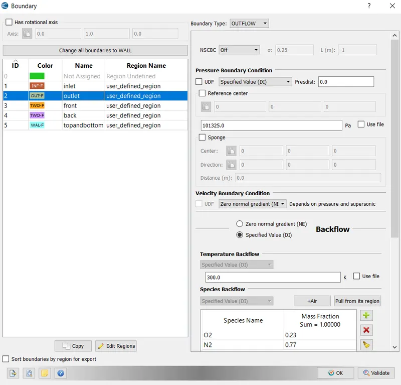
Outlet has been assigned an outflow boundary, with a initial pressure of 101325Pa.

Top and Bottom

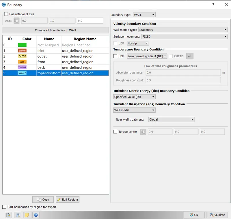
No slip boundary condition has been assigned to the topandbottom boundaries.

Front and Back

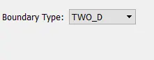
Front and back has been designated a 2D boundary type. Since the experimental length is infinite along these directions. So, Two-D boundary type has been assigned in these boundaries.

Turbulence Modelling

K epsilon model with the default parameters has been used for the present simulation. Although for accurate boundary layer simulation K-omega is more suitable, but for industrial application K - epsilon has been developed as it can converge large mesh size much easily with suitable boundary layer mesh size. Bounday layer modelling has not been done accurately here as it is beyond the scope of this project.

 

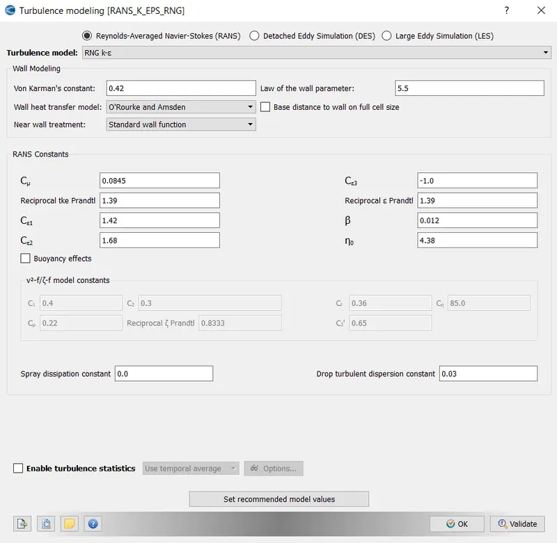
Grid Size

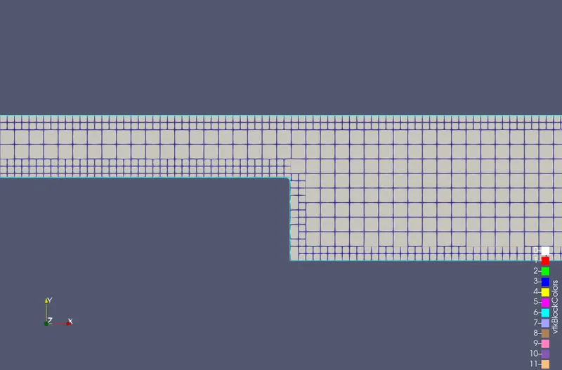
Grid size has been varied as described in the outline of the project.

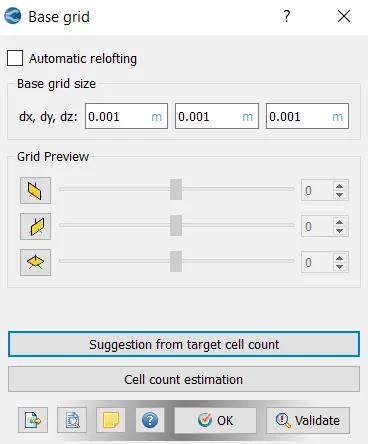
Embedding

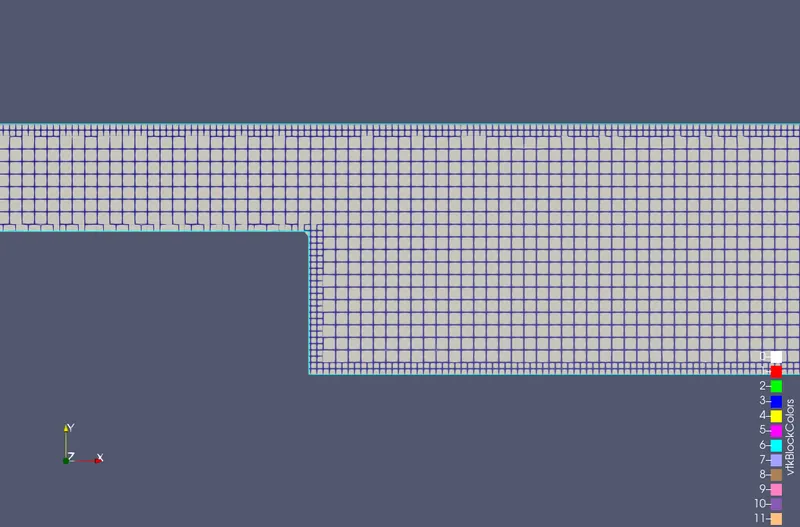
For boundary layer mesh refinement Embedding has been enabled with the following values.

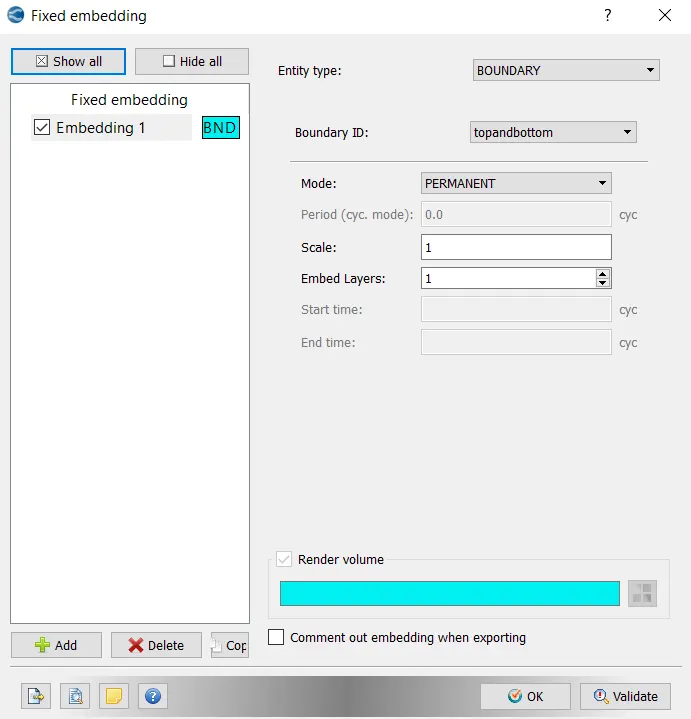
Post Variable

Following post variables has been marked for the output.

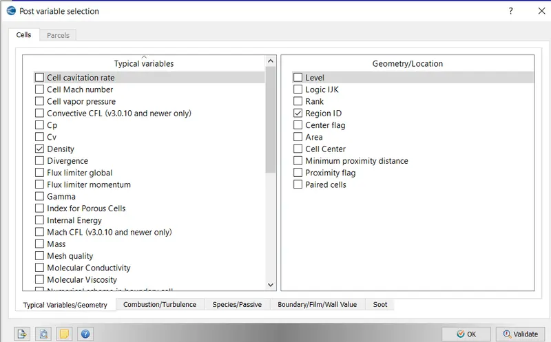
Output Files

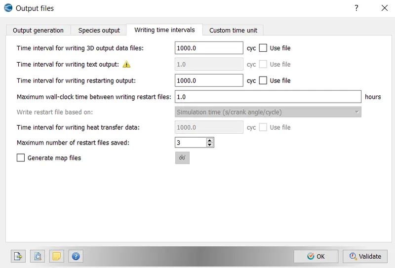
For decreasing the runtime of simulation, output files are being written at large intervals, Also, since we are more interested in steady state results, the in between results has very less significance.

Results and Discussion

Case 1:

Grid:

Contour Plot:

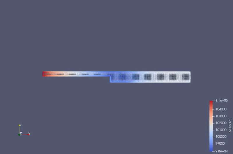
               Pressure: 

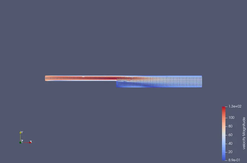
               Velocity:

Line plot at the boundaries:

               Total Pressure Plot:

               Average Velocity Plot:

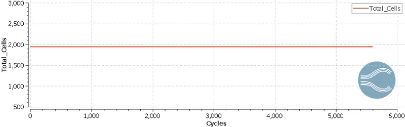
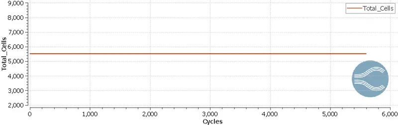
Cell Count:

Velocity Animation:

Case 2:

Grid:

Contour Plot:

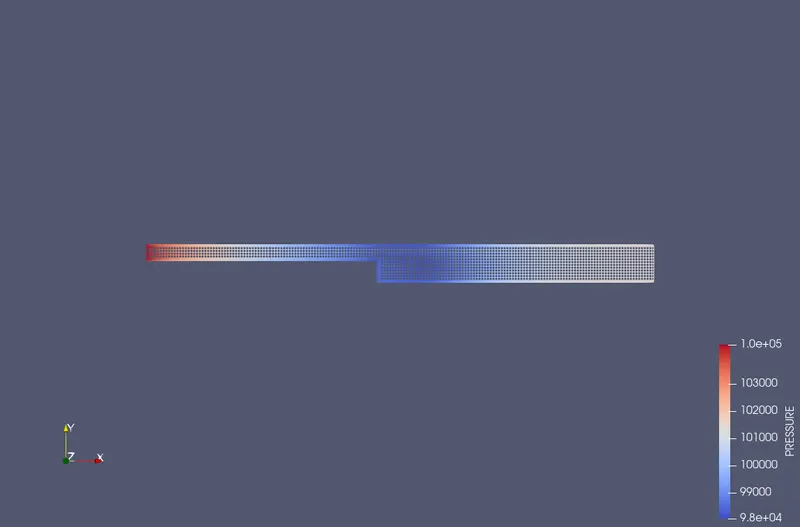
               Pressure:

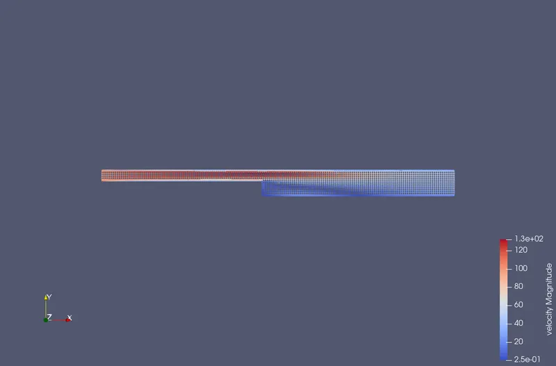
               Velocity:

Line plot at the boundaries:

               Total Pressure Plot:

               Average Velocity Plot:

Cell Count:

Velocity Animation:

 

Case 3:

Grid:

Contour Plot:

               Pressure:

               Velocity:

Line plot at the boundaries:

               Total Pressure Plot:

               Average Velocity Plot:

Cell Count:

Velocity Animation:

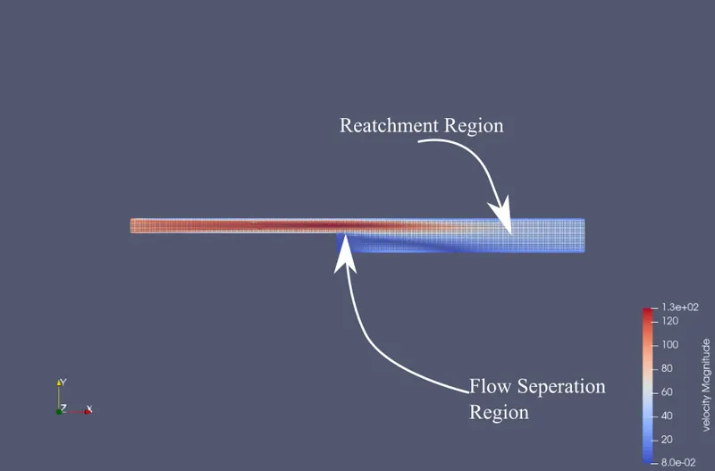
Region of Seperation and Attachment:

Conclusions:

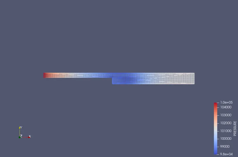
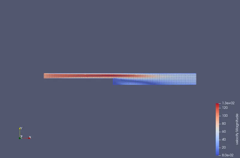
1. The pressure gradient between inlet and outlet leads to velocity in the direction of outlet. We can clearly see that as the fluid leaves past inlet the actual crossectional area of flow reduces within the first half of the volume, this leads to increase in flow speed. It happens cause of wall boundary layer of no slip condition.

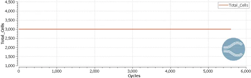
2. As before the change in grid size affects the cell count. Also, it remains constant for the entire simulation.

3. Change in grid size marginally affects the value of variables. It can be broadly studied in mesh independence study which is beyond the scope of this project.

4. In the step region, there is instant change in cross-section area of flow. This leads to abrupt variation in the pressure. It leads to formulation of low pressure zone and high pressure zone on the opposite boundaries. In the step region, as a consiquence of sudden pressure varion, recirculation happens. Later as the flow progresses, the phenomenon of reattachement is seen.