Week 3: Flow over a backward facing step
Given Data
back ward Facing in step geomentry
Turbulent solving
Steaty State
Boundary Condition
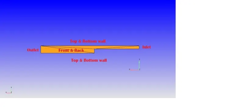
Volume- Air
inlet- 1101325 Pa
outlet-101325 Pa
Turbulent-`STD k-epsi`
SteatyState
Simulation time Parameter
End Time:15000 cycle
Initial Time step:1e-6
min Time step:1e-6
max Time step:1
Max convection CFL limit:1
Steaty state monitor
pressure-none
Solver parameter
Steady state solve control
Max convection CFL limit:0.5
Grid Control
Case1
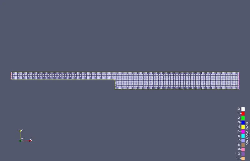
dx = dy = dz =2e-3m
Case 2
dx = dy = dz =1.5e-3m
Case3
dx = dy = dz =1.0e-3m
Fixed Embeded
Entity Type: Boundary
Boundary ID: Top & Bottom
Mode:Permanent
Scale:1
Embed Layer:1
Export input Data From Converge
Out Put
Case1
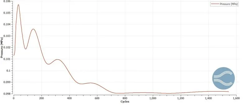
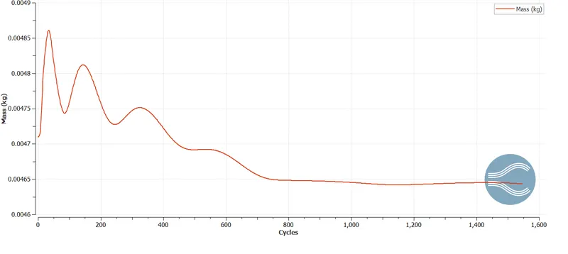
Output outlet condition in Converge
Pressure
Mass Flow
Mesh
Velocity
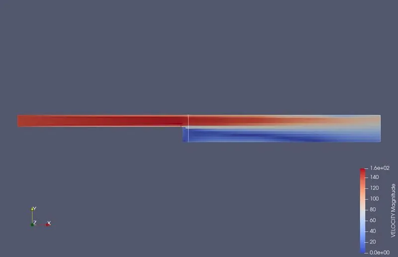
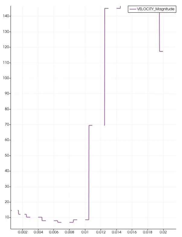
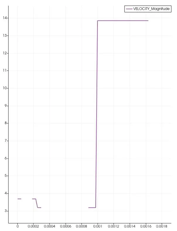
velocity vary in line plot
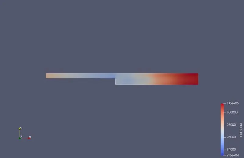
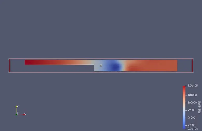
Pressure
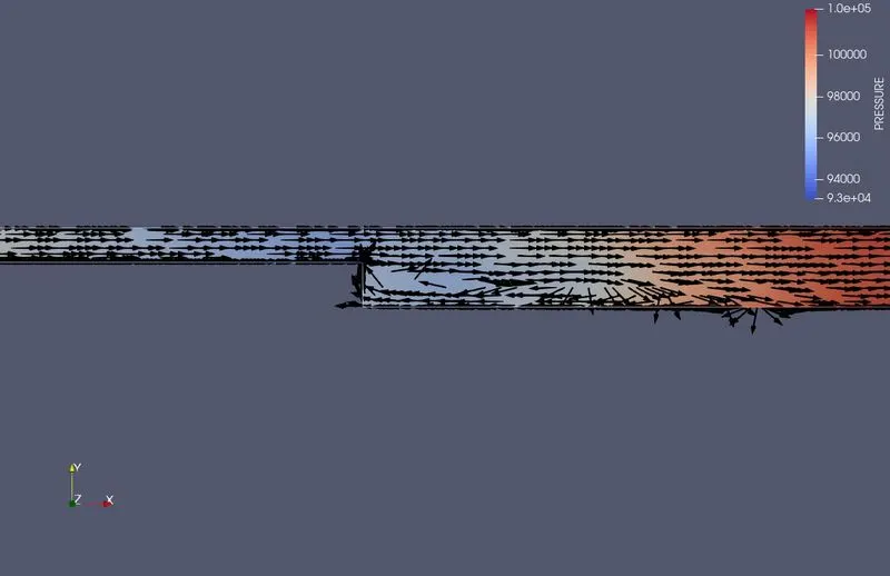
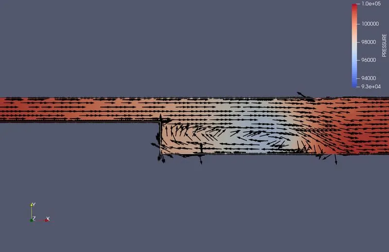
vector v f(P)
Case2
Output outlet condition in Converge
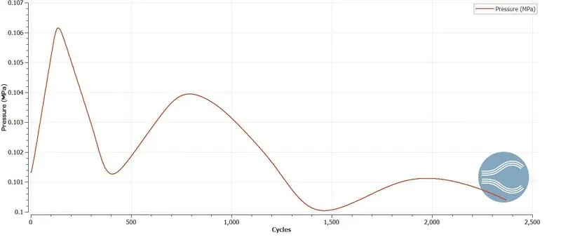
Pressure
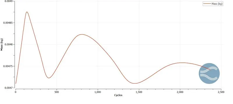
Mass Flow
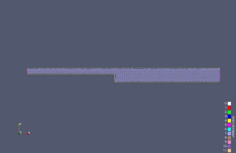
Mesh
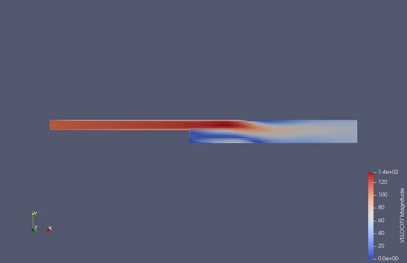
Velocity
plot over line
Pressure
vector v f(P)
Case3
Output outlet condition in Converge
Pressure
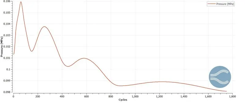
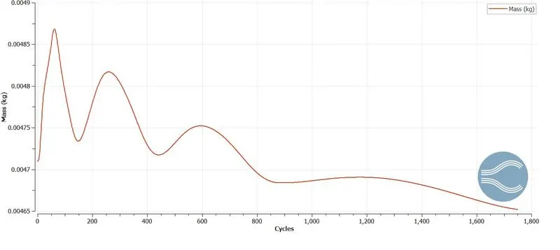
mass flow
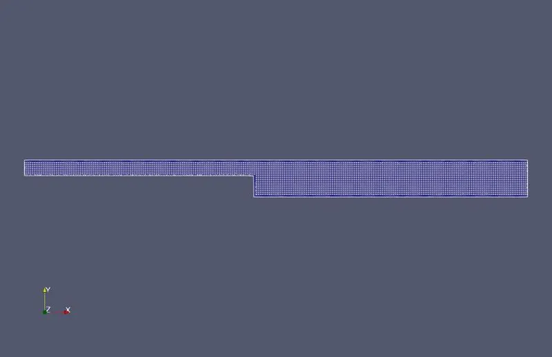
Mesh
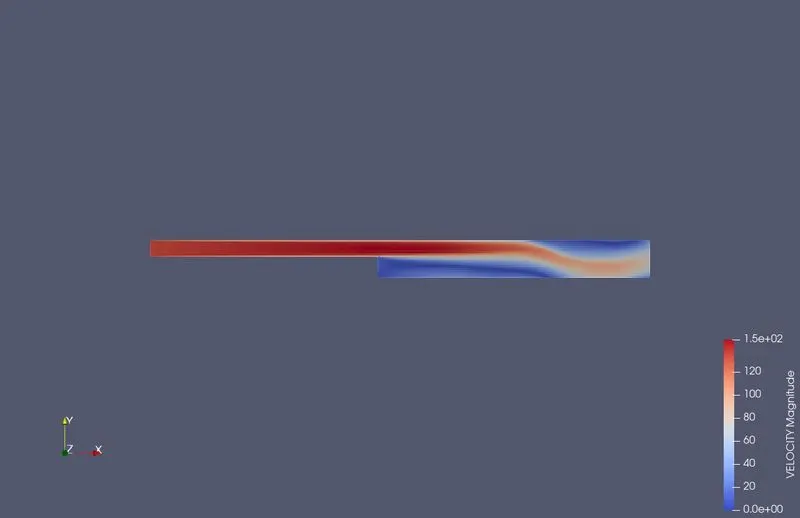
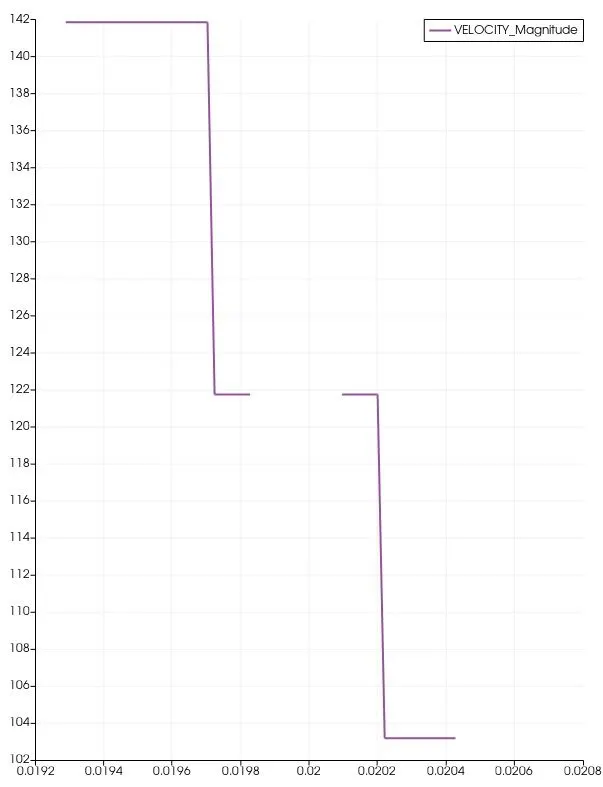
Velocity
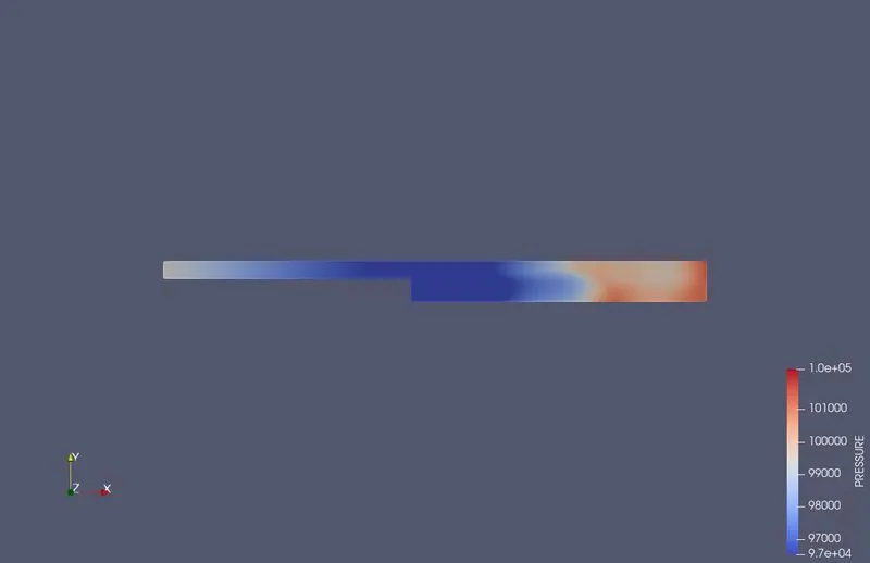
Pressure
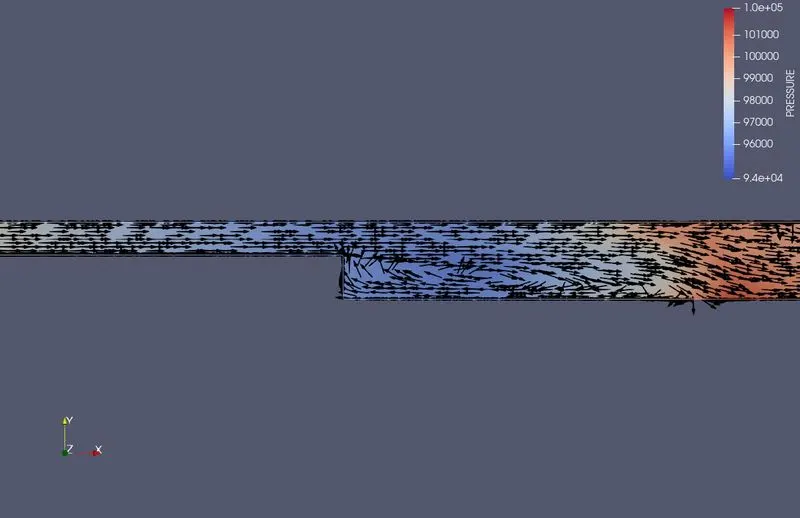
vector v f(P)
Conclution
From observation of three cases fine mesh case 3 1e-3 capture eddies in the flow step so there is back flow and swirl generation at step region where decrease in Pressure after at it obtain maximum Pressure (1e-5). in step region almost velocity decreases even tends to be nullified This is due to changes of geomentry from converge to Divergent Area.
solving for case 3 is more computer expensive compare to other case this due to lesser mesh size and more cells