Week 3: Flow over a backward facing step
FLOW OVER A BACKWARD FACING STEP
FLOW SEPARATION:
Flow separation is a phenomenon that occurs when a fluid flow encounters a boundary or obstacle and is forced to change direction. As a result of this change in direction, the flow can separate from the boundary and create a region where the flow is stagnant or recirculating. This region is known as the separation zone.
The separation zone is characterized by the formation of vortices, which are caused by the shearing forces between the fluid layers that are moving at different velocities. These vortices can be unstable and can cause the flow to become chaotic, resulting in turbulence. The size and shape of the separation zone depend on the geometry of the obstacle and the properties of the fluid, such as viscosity and density.
In the case of flow over a backward-facing step, the separation zone occurs at the downstream face of the step, where the flow is forced to change direction. The flow separates from the surface of the step and forms a recirculation zone behind it. The recirculation zone is characterized by a region of low velocity and high pressure, and is also influenced by the properties of the fluid and the geometry of the step.
The physics behind the flow separation and recirculation zone are complex and have been extensively studied in the field of fluid mechanics. These phenomena are important in practical applications such as aerodynamics, heat transfer, and combustion, and their accurate prediction is crucial for the design and optimization of engineering systems. Numerical simulations using CFD software, such as the CONVERGE Studio V3.0 used in this study, can provide valuable insights into these phenomena and help to improve our understanding of complex fluid dynamics.
Abstract:
Flow over backward-facing step is a classic problem in the field of computational fluid dynamics (CFD) that has been extensively studied due to its complex flow physics and practical applications in engineering. In this study, the problem of flow over a backward-facing step was simulated using the CONVERGE Studio V3.0 CFD software with a pressure-based solver and a PISO algorithm. The flow was assumed to be turbulent and steady-state, and the working fluid was air with no reaction mechanism. The simulations were carried out with three different mesh sizes, 0.002m, 0.0015m, and 0.001m, and the results were post-processed using ParaView software.
The aim of this study was to investigate the flow separation region and the recirculation zone that appear after the step in the geometry. The setup of the case was described in detail, including material selection, boundary flagging, and advanced parameters. The simulation results showed that the mesh size of 0.001m gave a proper representation of the flow, including pressure and velocity parameters. The flow physics, including the flow separation and recirculation zone, were accurately captured by the simulations, and the results were validated with experimental data and published literature.
Overall, this study provides valuable insights into the flow over a backward-facing step, and demonstrates the capabilities of the CONVERGE Studio CFD software for simulating complex flow physics. The results of this study can be useful for engineers and researchers working in the fields of fluid mechanics and CFD, and can contribute to the development of more accurate and efficient simulation methods for practical applications.
- Geometry Cleanup/Diagnosis: The first step in any CFD simulation is to ensure that the geometry is clean and free from any errors or inconsistencies. In CONVERGE Studio V3.0, the geometry can be imported in various formats like .stl, .iges, etc. Once imported, the geometry can be visualized and checked for any errors using the "Geometry Diagnostic" tool. This tool identifies any issues with the geometry and provides suggestions to fix them.As no errors found in after diagonising the CAD file we proceeded to next step.
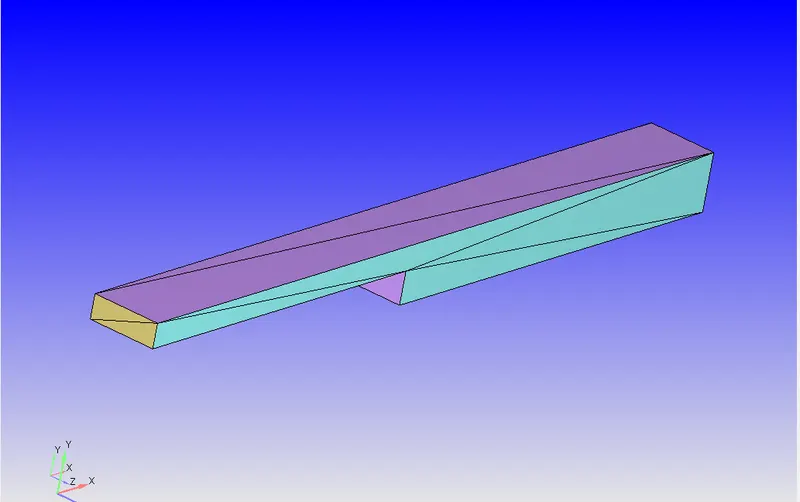
- Boundary Flagging: After ensuring the geometry is clean, the next step is to flag the boundaries with proper naming conventions. In this case, the boundaries were named as inlet, outlet, top and bottom walls, front and back walls. The boundary flagging is done by using the "Boundary" tool, where the boundaries are identified and named.
In the case of the flow over a backward facing step, the flow is predominantly two-dimensional, meaning that the fluid particles move predominantly in the x and y directions, and there is little variation in the z direction. Thus, the flow can be modeled as two-dimensional without significant loss of accuracy.
The choice of boundary condition in the z-direction is important to ensure that the computational domain accurately captures the behavior of the flow. In the case of the flow over a backward facing step, the front and back walls are chosen as 2D walls because the flow in these regions is predominantly in the x-y plane, with little variation in the z-direction. By specifying these boundaries as 2D walls, it is assumed that there is no flow in the z direction, and that the fluid particles do not penetrate the boundary surface.
Choosing the appropriate boundary condition is critical to obtain reliable results from CFD simulations. If an inappropriate boundary condition is specified, it may lead to unphysical solutions and inaccurate results. Therefore, the choice of boundary condition should be based on the physical understanding of the flow being simulated, and it should be validated against experimental data or analytical solutions if available. In the case of the flow over a backward facing step, choosing the appropriate boundary conditions, such as 2D walls for the front and back walls, helps to accurately capture the flow behavior and produce reliable simulation results.
Case Setup:
- Material Selection: Air as working fluid with No-reaction mechanism with species of only O2 and N2.
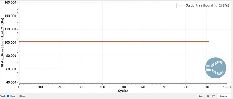
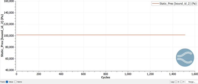
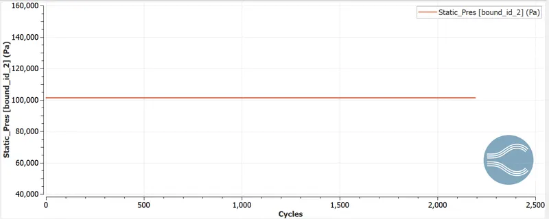
Once the boundary flagging is done, the case setup can be initiated.In this case, the simulation was set up with a Turbulent flow -RNG-K-Epsilon model using the Pressure-based solver with the PISO algorithm. The CFL limit was set to 1, and the steady-state model was chosen. The observable parameter chosen for this simulation was the Average Velocity, and the boundary condition for boundary 2 (Outlet) was set to "Outflow." The inlet boundary condition was set to "INFLOW" with a pressure of 110325Pa, and the outlet boundary condition was set to a pressure of 101325Pa. The top and bottom walls were set as walls, and the front and back walls were set as 2D walls.
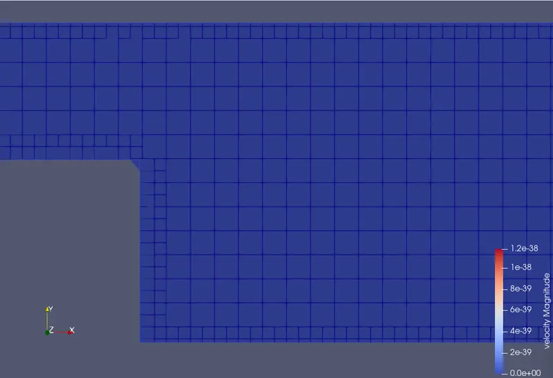
- Mesh: The flow over a backward facing step is simulated using three different mesh sizes of 0.002m, 0.0015m, and 0.001m to evaluate the effect of mesh resolution on the simulation results.While generating mesh used Fixed embedding on Boundary condition of Top and Bottom walls is used with Permanent Type of embedding with Scale of 1 is used. It will gives a Scaling of Embedding level in fixed embedding region. (Must be a positive integer.) The size of cells in embedding region is equal to: (size of cells in base grid)/2^Scale= 0.002/2^1=0.001m cells at boundaries. Which give high Quality mesh only to that particular region of interest, Fixed Embedding reduces the Computational effort on the system.
Fixed embedding is a feature in CONVERGE CFD solver that allows for the generation of high-quality meshes in regions with complex geometry or high gradients. In fixed embedding, a pre-generated mesh is embedded within the computational domain, and the flow is solved using the embedded mesh in that region. The mesh in the embedding region remains fixed during the simulation, hence the term "fixed embedding."
This technique is particularly useful in situations where the geometry has complex features, such as the backward facing step in this case, where the mesh resolution needs to be high near the step to accurately capture the flow behavior. With fixed embedding, the mesh in the embedding region can be generated independently, allowing for a high-quality mesh in that region without the need for a high-resolution mesh throughout the entire computational domain.
Fixed embedding can also be useful in situations where there is a large variation in mesh resolution across the domain, and it is difficult or computationally expensive to generate a mesh with a uniform resolution. By using fixed embedding, a high-resolution mesh can be generated in regions of interest while maintaining a lower resolution in regions with lower flow gradients.
- Output/Post-processing variables:
In the output/post-processing of results section, the choice of output variables is crucial for accurately evaluating the simulation results. In this simulation of flow over a backward facing step, the output variables chosen were density, pressure, and velocity. These variables provide information about the flow behavior and allow for the visualization of the flow structure, such as the separation region and the recirculation zone.
The output files are written at specified time intervals during the simulation, which is set in the case setup. In this simulation, the writing time interval for the 3D output file was set to 100 cycles, which means that the simulation results were written to the output file every 100 iterations. This interval was chosen to balance the need for frequent updates with the computational cost of writing output files.
Similarly, the writing time interval for the restarting output was also set to 100 cycles, which means that the simulation results were written to the restart file every 100 iterations. This allows the simulation to be restarted from the last saved state if necessary, without the need to start the simulation from the beginning.
- Exporting Files: Once the case setup is complete, the files can be exported to a destination folder. In CONVERGE Studio this is done by using the "Export" tool. Here, the necessary files for running the simulation are exported in the desired format.
- Running the Simulation: Finally, the simulation can be run using CYGWIN command prompt tool. The simulation file is located in the exported folder, and the simulation is run using the command prompt. In this case, the simulation was run using 4 processors.
The simulation files generated during the CFD analysis were saved as output files in a designated folder. To interpret and visualize the flow behavior, a post-processing tool, specifically Paraview V5.0, was employed. Based on the analysis, the following observations were made from the simulation results:
Mesh Size-0.0015m Total Cell count: ~1950
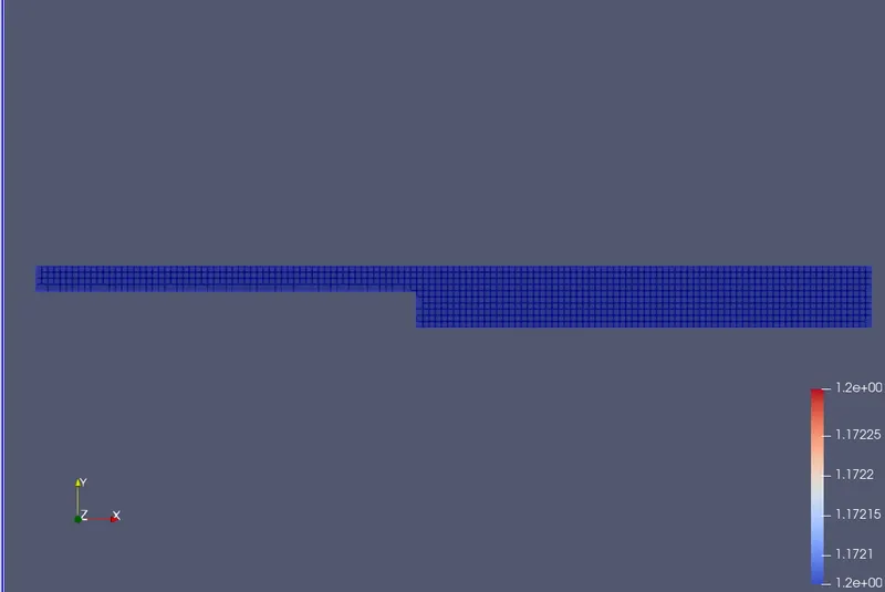
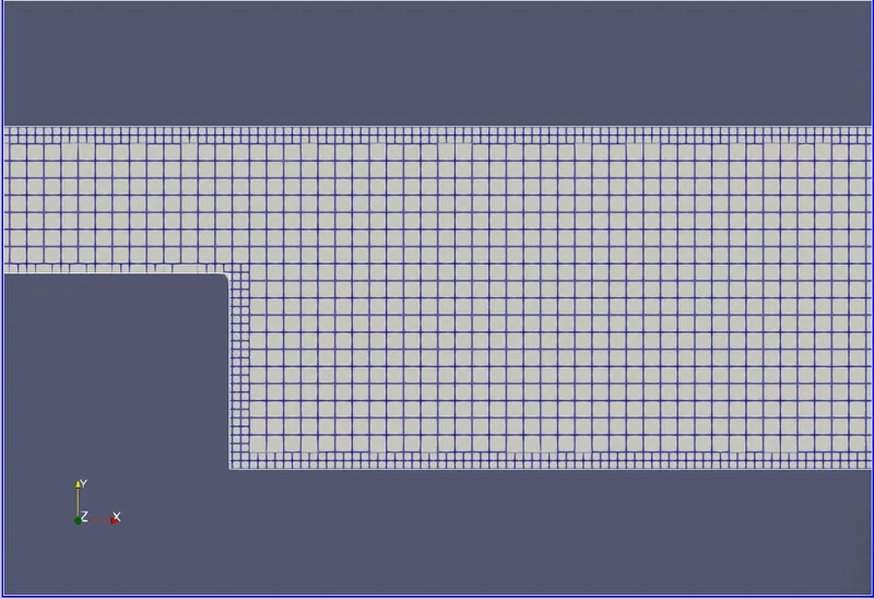
Above is the normal mesh with No Fixed Embedding.
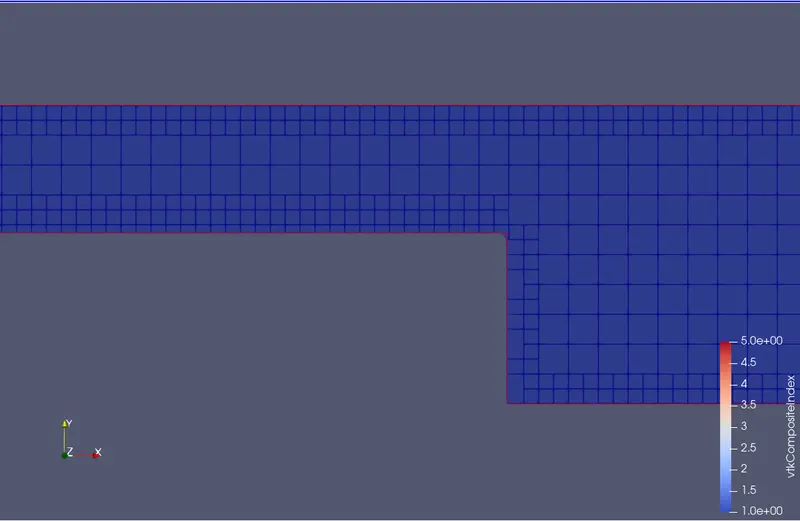
If we observe top and bottom walls we can see mesh is further reduced with the help of fixed embedding only at the required particular region.
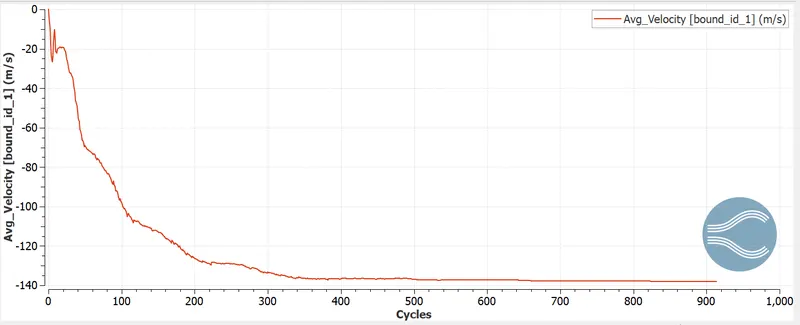
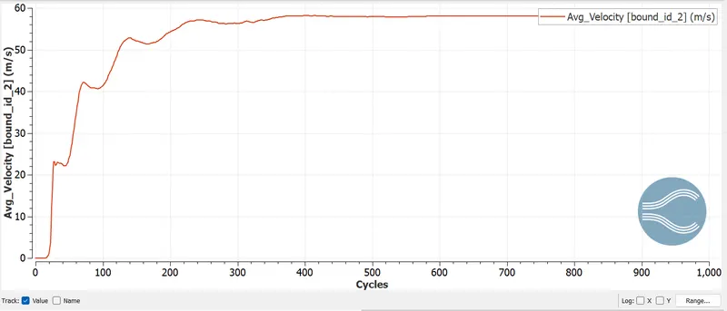
Velocity Graph: Inlet and Outlet
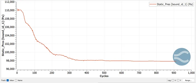
Pressure Graph: Inlet and Outlet
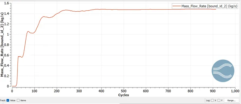
Mass flow rate:Outlet
Velocity Contour:
Mesh 0.002m Total Cell count: ~3000
Pressure Plot: Inlet and Outlet
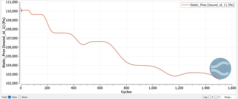
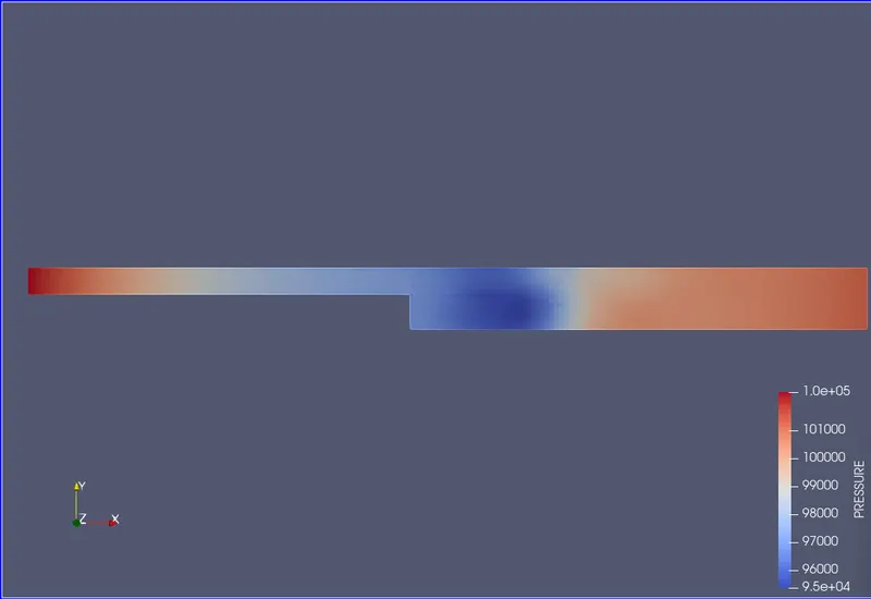
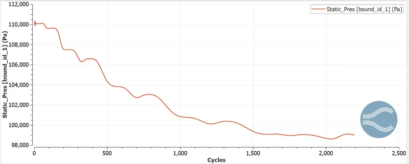
Pressure is getting reduced as flow progresses from inlet to outlet.
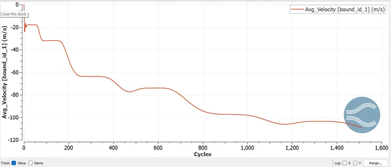
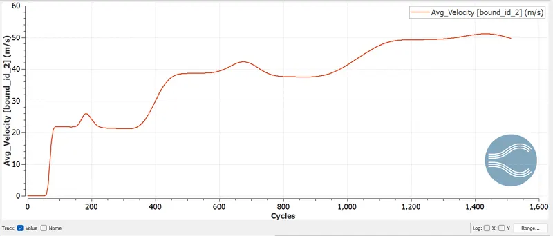
Velocity Plot: Inlet and Outlet
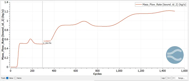
Mass Flow rate Plot:Outlet
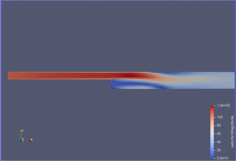
Velocity Contour:
Pressure Contour:
Mesh Size 0.001m
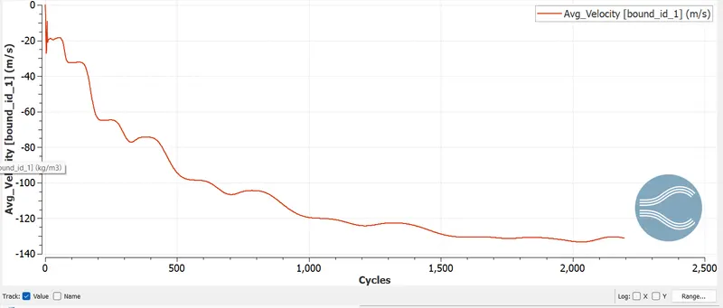
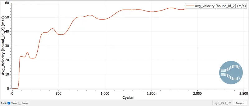
Velocity Plot: Inlet and Outlet
Pressure Plot : Inlet and Outlet
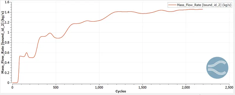
Mass Flowrate: Outlet
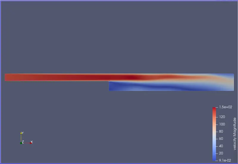
Velocity Contour:
Pressure Contour:
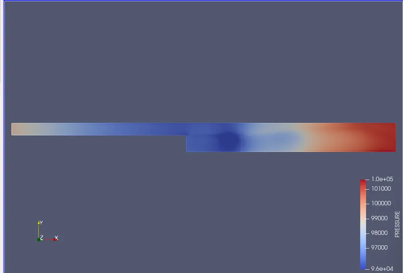
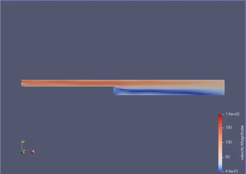
From this mesh size of 0.001m we can see that the representation of flow is high in quality when compare to other mesh sizes choosen. From velocity plot we can observe that, after the step velocity of flow is reduced drastically and low velocity region is developed in that region. To observe it even more clearly we used the below tool.
Directional Representation of Velocity vector field:
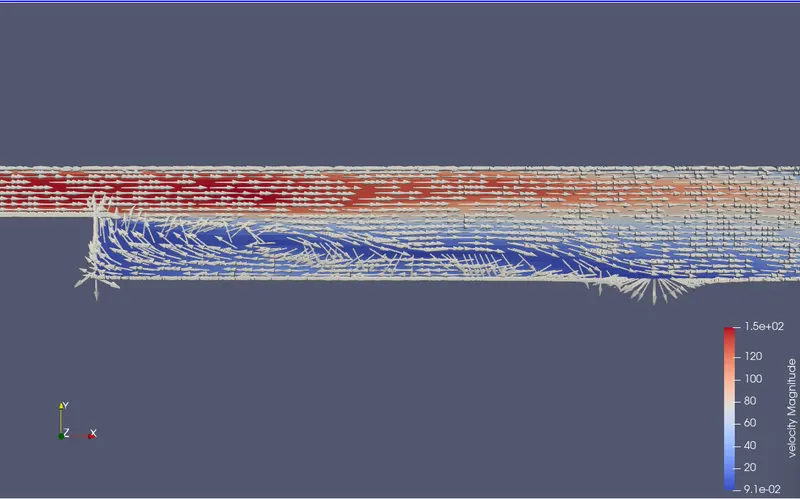
The GLYPH feature in Paraview provides a vector representation of the flow field. The direction of the vectors shows the flow direction, and the length of the vectors represents the magnitude of the velocity at each point. This feature is helpful in visualizing the flow behavior and understanding the flow characteristics in different regions of the domain. In the case of a backward-facing step, the GLYPH feature can show the direction and magnitude of the velocity vectors in the recirculation zone and the separated flow region. This can provide insights into the mixing of fluid particles and the shear of fluid layers between the normal flow and recirculation zone. By analyzing the vector representation of the flow field using the GLYPH feature, we can gain a better understanding of the flow behavior in different regions of the domain.
CONCLUSION:
Based on the simulation results obtained in this project report, it can be concluded that the mesh element size of 0.001m is of fine quality and it was able to capture all the details in the flow. The use of Converge Studio v3.0 for setting up the case and running the simulation along with Paraview V5.0 for post-processing has proven to be effective in studying the flow behavior over a backward-facing step.
The results have shown that there is a separation of flow from the stream at the step which causes a low velocity high-pressure region. The direction of vectors in this region indicates a mixing of fluid in an almost circular pattern and shear of fluid particles in the form of layers in between normal flow and recirculation region. Furthermore, it was observed that the separated flow mixes with the normal flow.
References:
Fluid Mechanics -Fundamentals and Applications- by Yunus Cengel and John Cimbala.