Week 3: Flow over a backward facing step
Aim:
To perform a Backward facing step simulation using Converge and postprocess the result in Para view.
Objective:
- Run 3 simulations and compare the results between all the 3 simulations.
- 3 different base mesh sizes are,
Once you have the base setup ready, run the case for three different base mesh sizes
- dx = dy = dz =2e-3m
- dx = dy = dz =1.5e-3m
- dx = dy = dz =1.0e-3m (If this is too much for your PC, use 1.2e-3m)
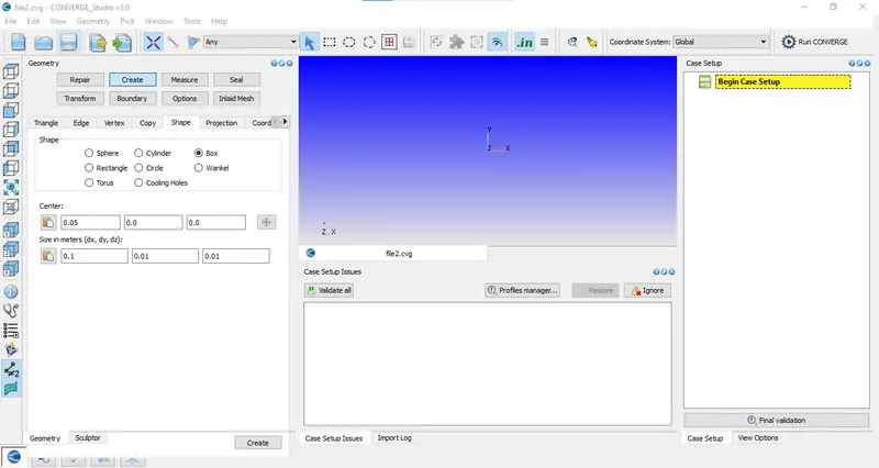
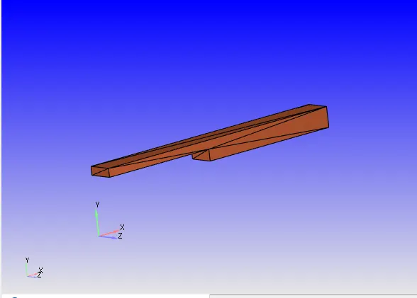
Geometry import
- Download the file from the download folder
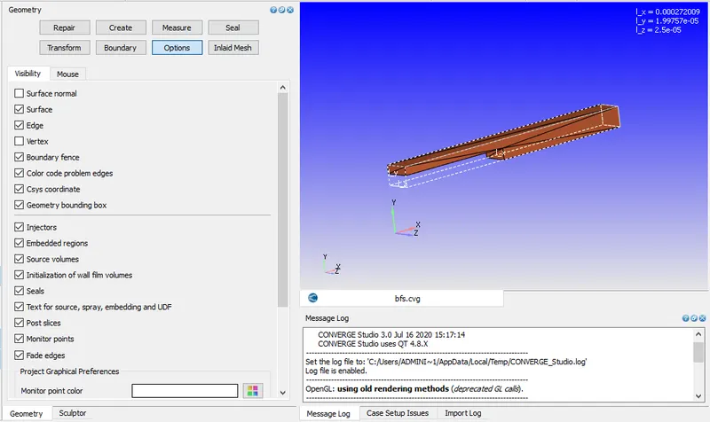
Geometry bounding box
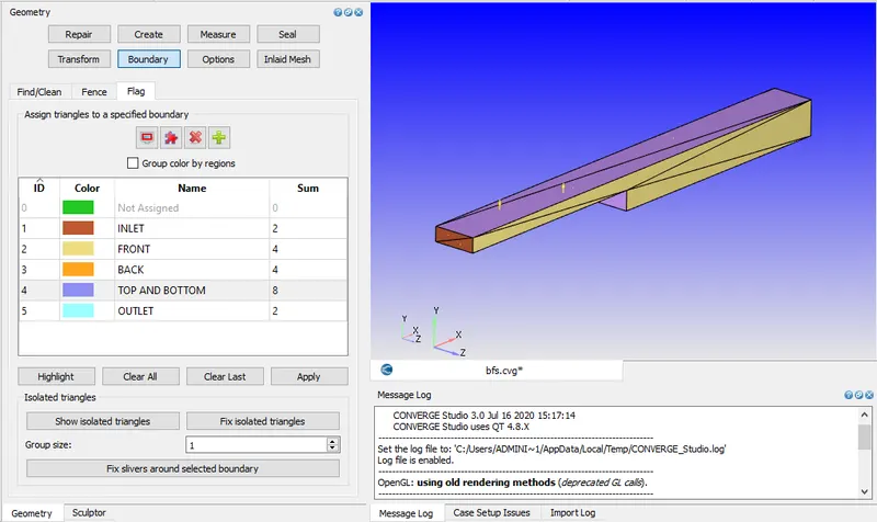
Boundary condition
Click on boundary and Create boundary
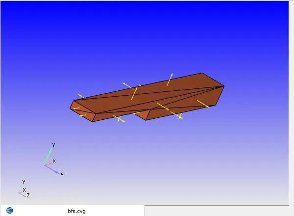
Check normal vector
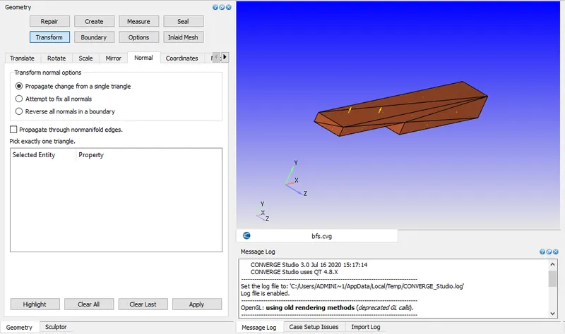
Again geometry- transform-normal/select the any one surface of triangle then click apply to avoid fatal error go to transform-rotate-select entire surface- rotate by 90 degree about x-axis then apply
Transform
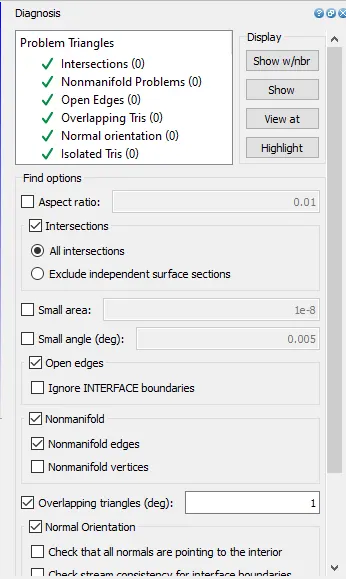
Diagnosis dock
Before proceeding the error in geometry for that
View tab-diagnosis dock-default setting-select the find
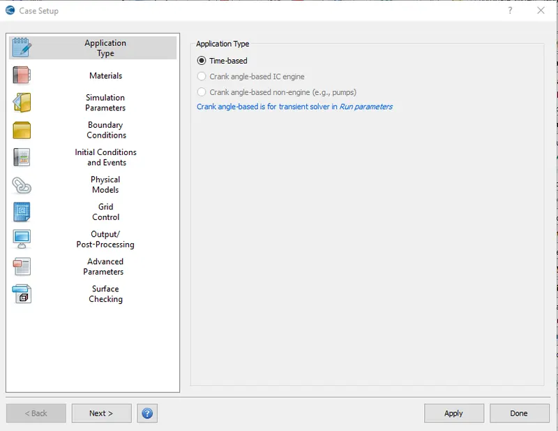
Case Setup:
Application Type = Time-based
Materials -
Predefined mixtures = Air
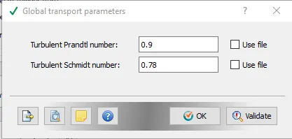
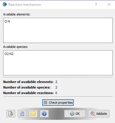
Select ‘Gas Simulation' & 'Reaction Mechanism
Material
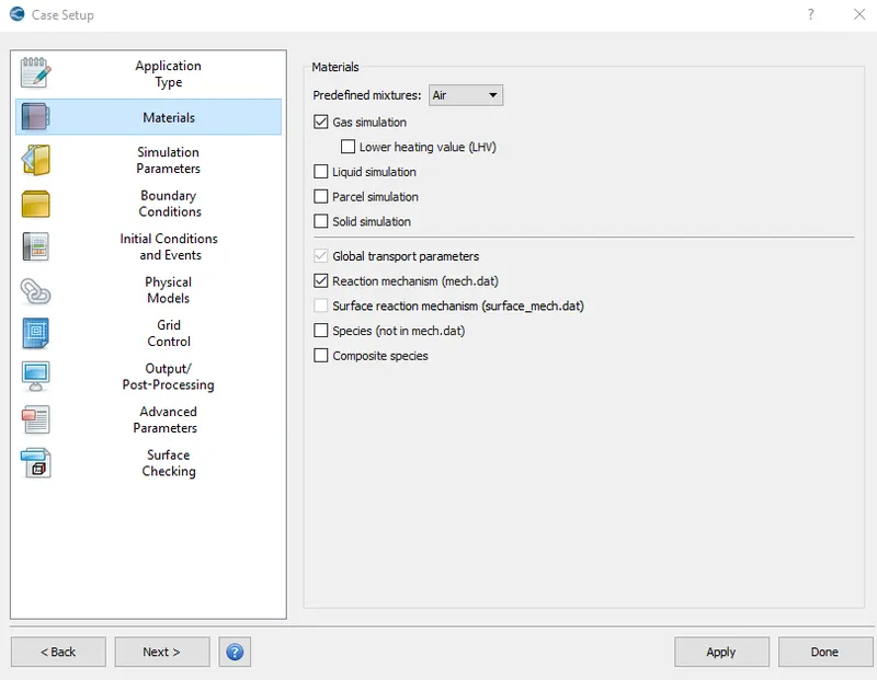
Gas simulation
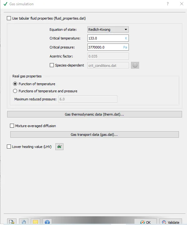
Global transport parameters
Reaction Mechanism
Simulation Parameters-
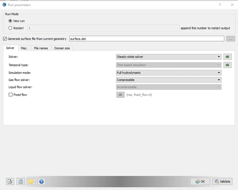
In Run Parameters two main things to be considered: -
select the following solver settings.
Go to Misc. > uncheck UseSharedMemory and click on Steady-State Monitor.
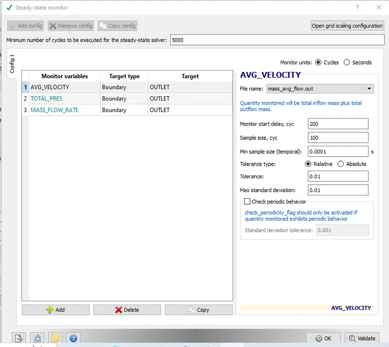
Steady-State Monitor:
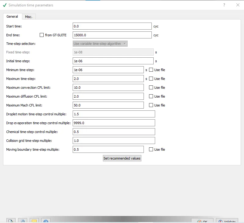
Simulation Time Parameters: -
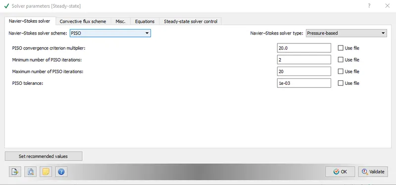
Solver Parameters [Steady-State]-
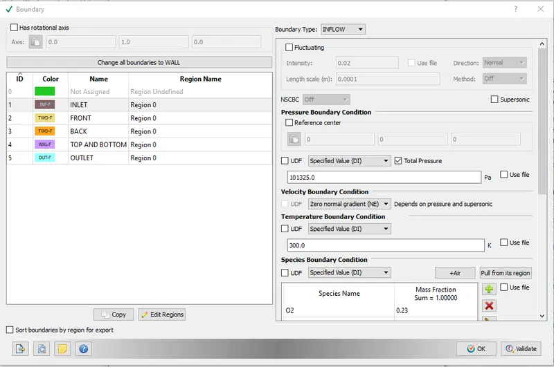
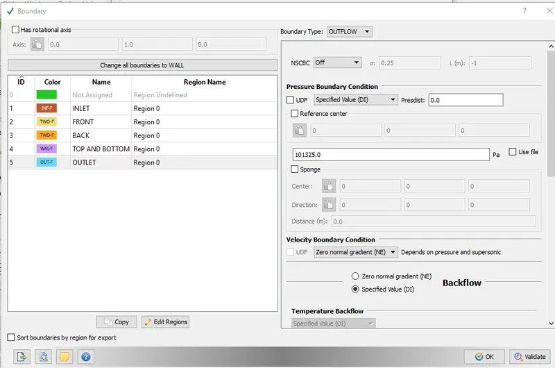
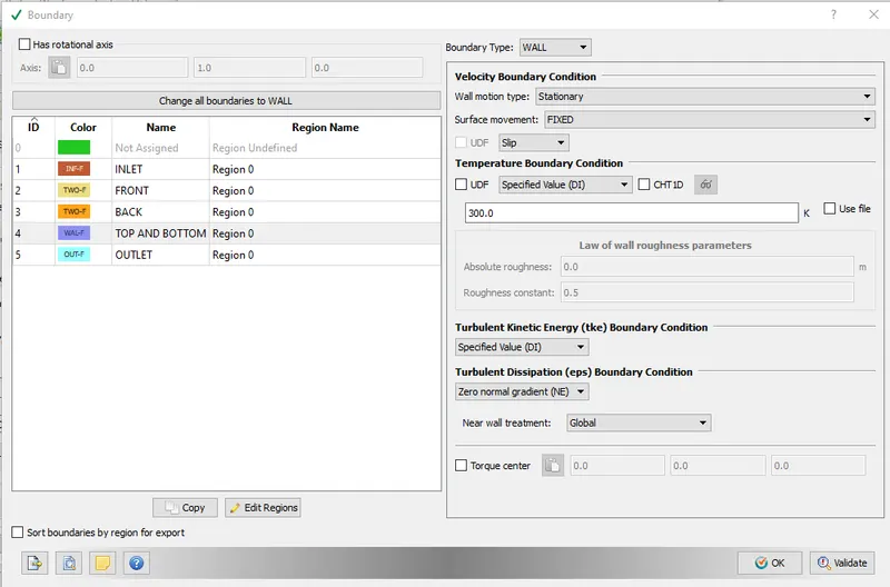
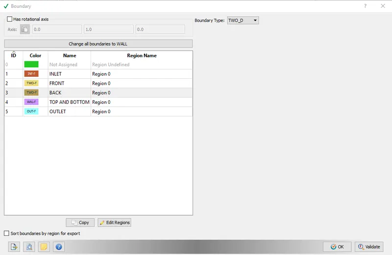
Boundary Conditions-
Boundary:
Inlet
Outlet
Top Bottom -Wall
For front2D and bacK2D - Boundary type: TWO_D
Initial Conditions and Events: -
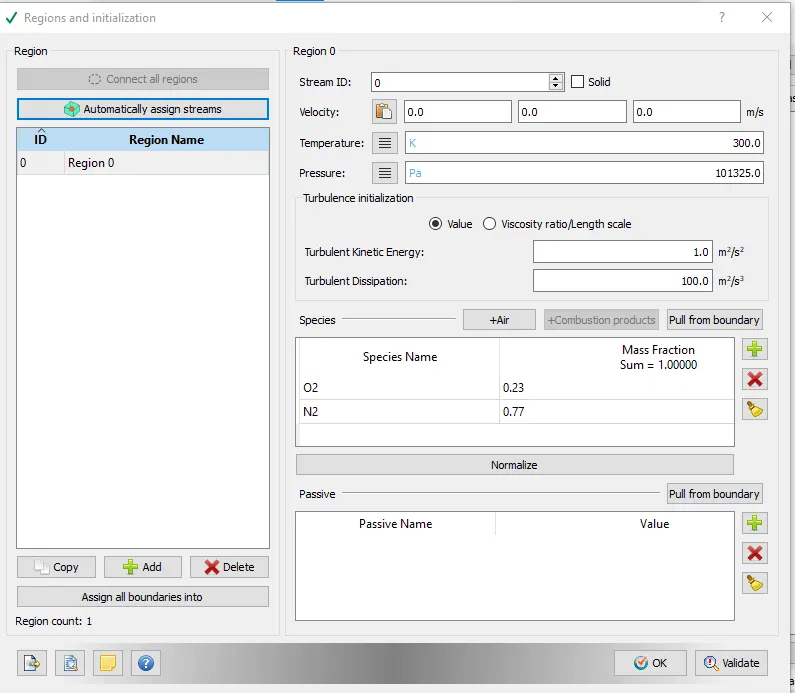
Regions and Initialization:
Physical Model
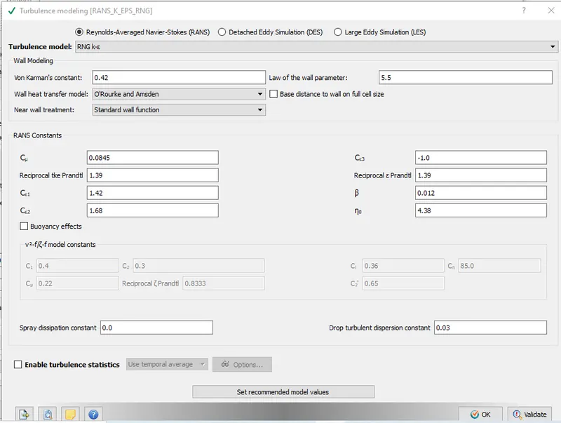
Turbulence Model
Grid Control: -
Base Grid:
- dx = dy = dz =2e-3m
- dx = dy = dz =1.5e-3m
- dx = dy = dz =1.0e-3m (If this is too much for your PC, use 1.2e-3m)
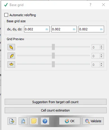
Note: change base grid size according to your setup
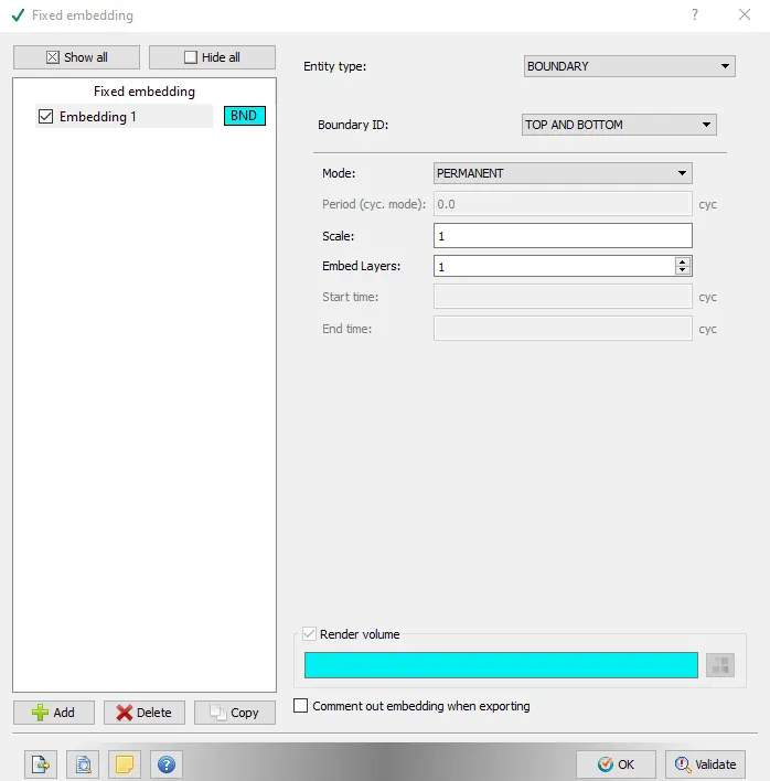
Fixed Embedding
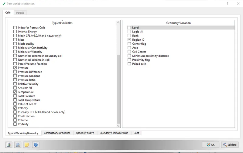
Post-Processing: -
Post Variable Selection:
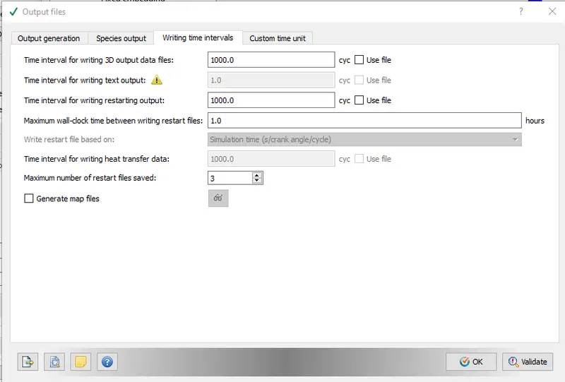
Output Files:
Case setup
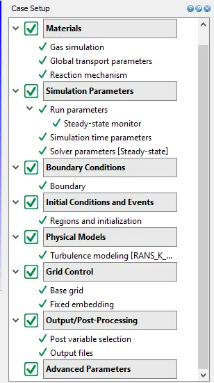
- With this setting up of the case is completed.
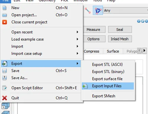
- Now go to File > Export > click on Export Input Files.
- select the destination folder (channel test) to save the data.
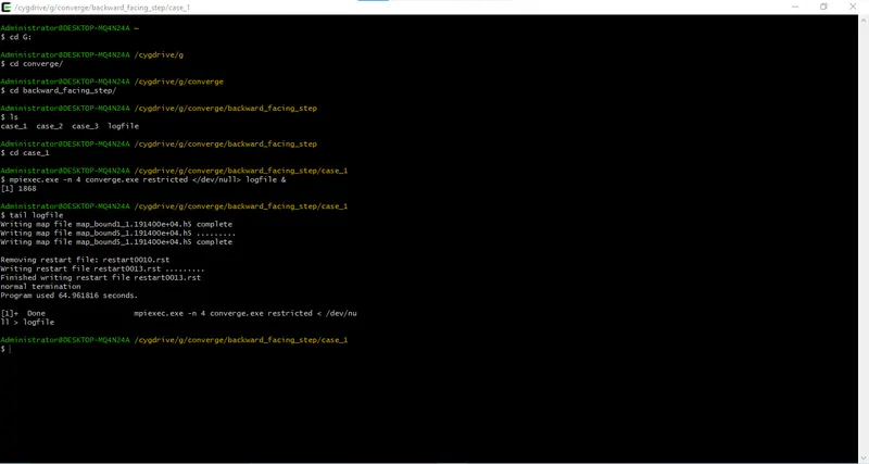
Solving: (solver for converge & executable for Cygwin64)
Results
Case 1: dx = 2e-3m, dy = 2e-3m, dz = 2e-3m
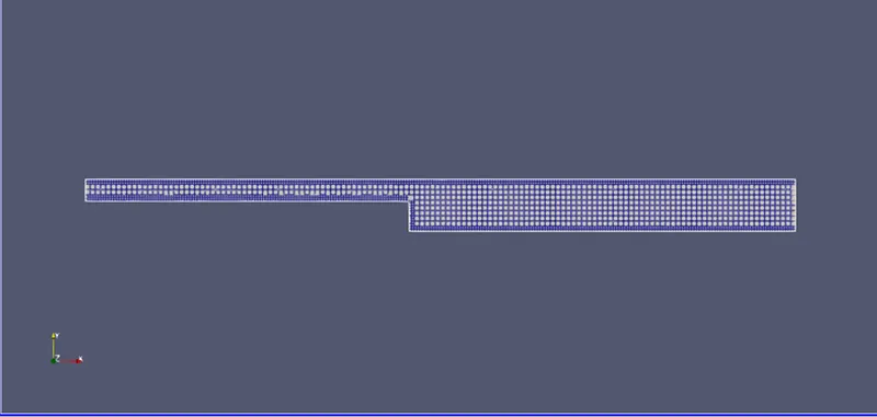
Mesh
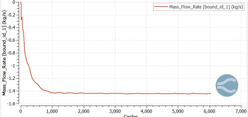
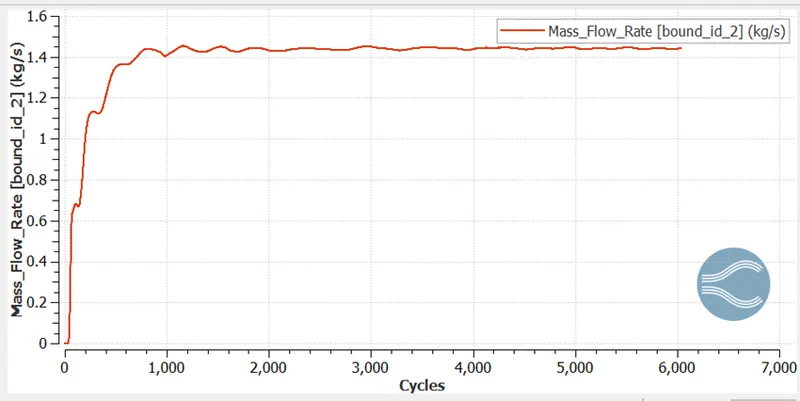
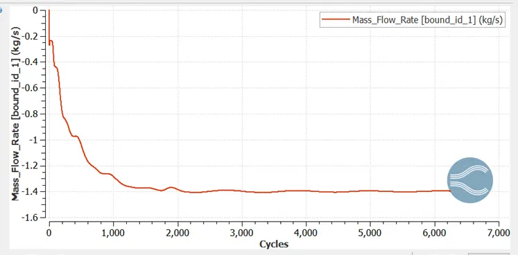
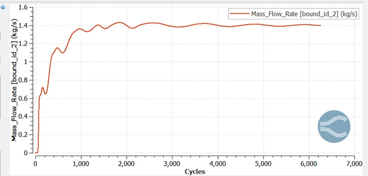
Mass flow rate
Inlet
Outlet
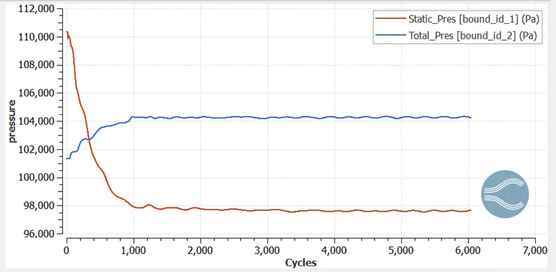
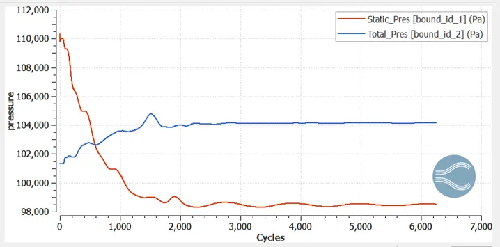
Pressure plot
Inlet And Outlet
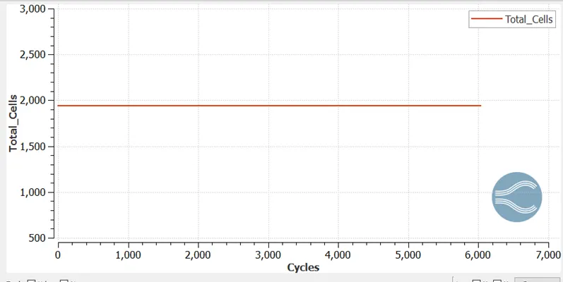
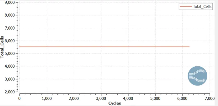
Total cells
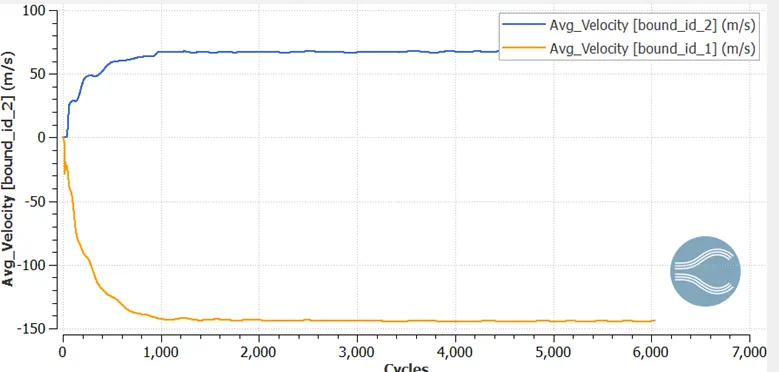
Velocity plot
Inlet And Outlet
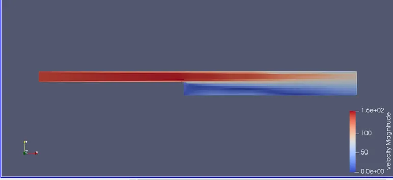
Velocity contour
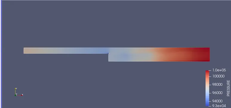
Pressure contour
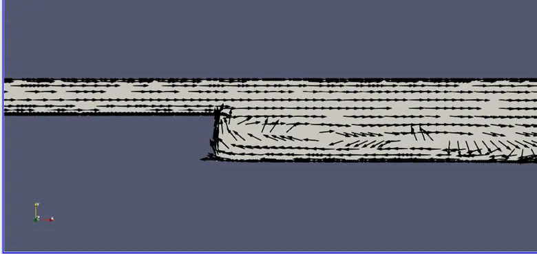
Velocity vector near recirculation
Case 2 : dx = 1.5e-3m, dy = 1.5e-3m, dz = 1.5e-3m
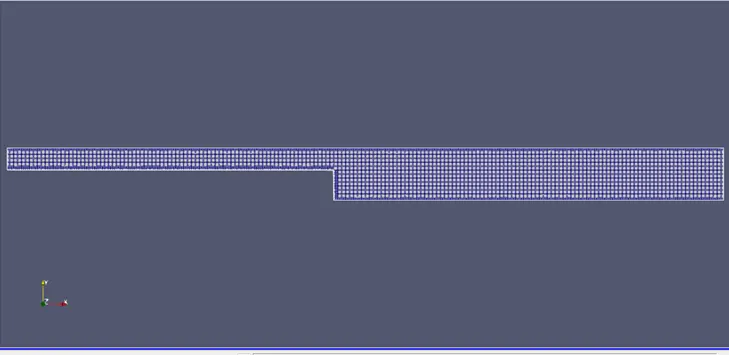
Mesh
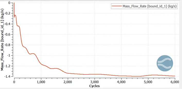
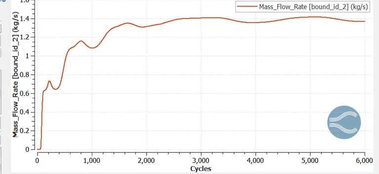
Mass flow rate
Inlet
Outlet
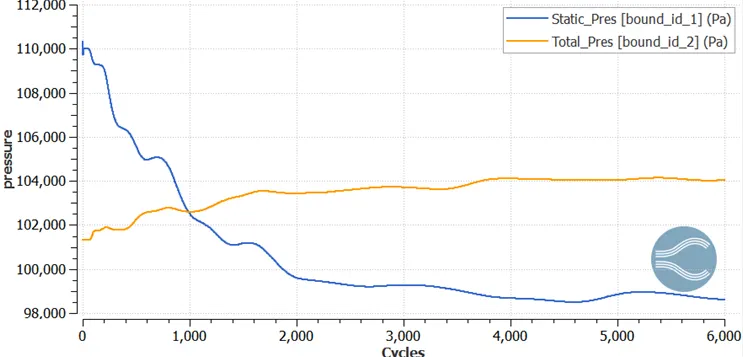
Pressure plot
Inlet and Outlet
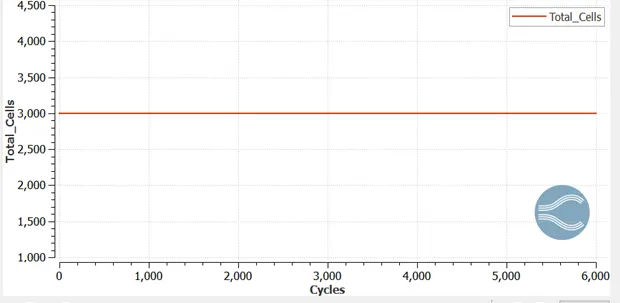
Total cells
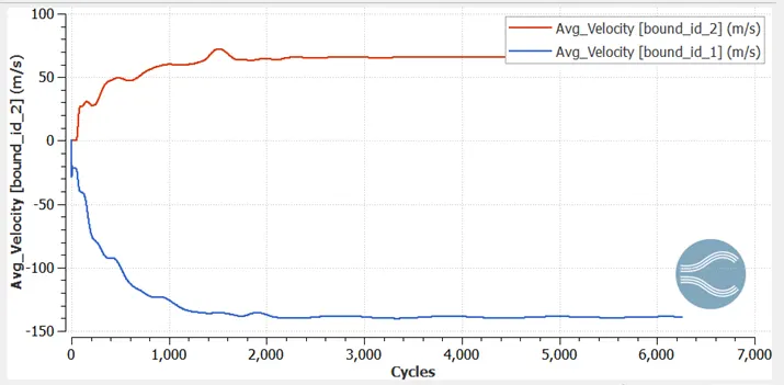
Velocity plot
Inlet and Outlet
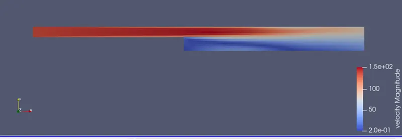
Velocity contour
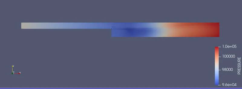
Pressure contour
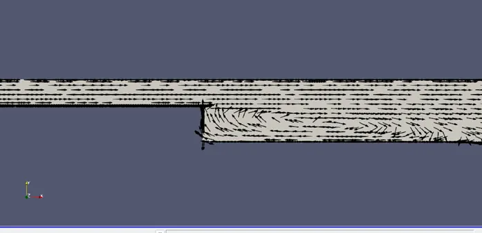
Velocity vector near recirculation
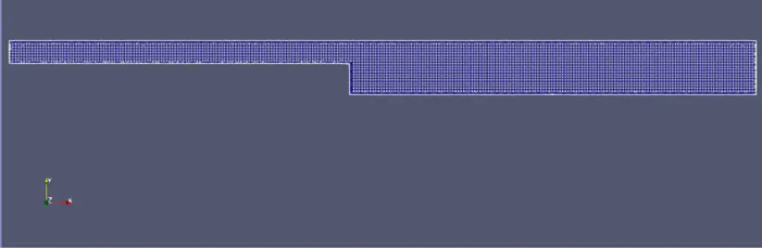
Case 3 : dx = 1e-3m, dy = 1e-3m, dz = 1e-3m
Mesh
Mass flow rate
Inlet
Outlet
Pressure plot
Inlet And Outlet
Total cells
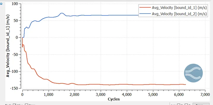
Velocity plot
Inlet and Outlet
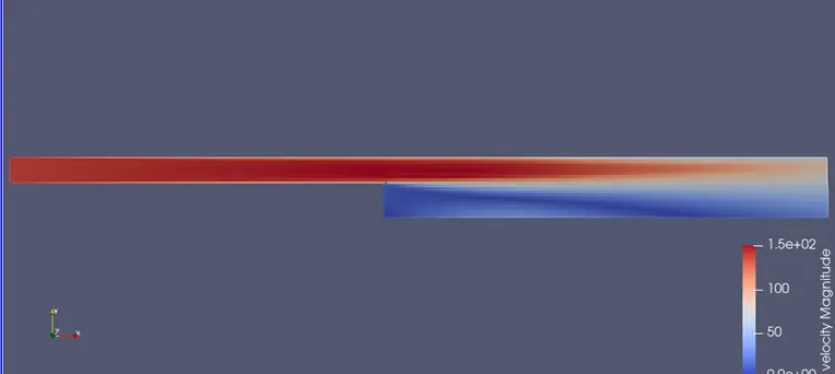
Velocity contour
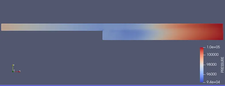
Pressure contour
Velocity vector near recirculation
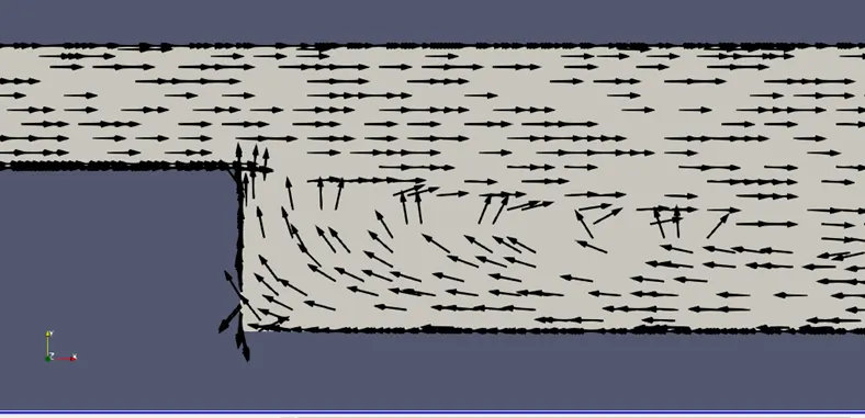
Flow separation:
- This is taking place at the back of the step where area is increased
- Due to positive pressure gradient created at this zone, the flow start moving backward
- As a result, the flow separates and a recirculation region is formed due to flow in opposite direction. This is also called Wake Region
Conclusion:
- Three simulations were run with different grid size and gives a necessary plots and contour
- With decrease in grid size means finer mesh the contours became smoother and more accurate results were found
- Fixed embedding gives finer mesh near the wall boundaries and its help for capturing physics nears the wall