Week 3 - External flow simulation over an Ahmed body.

AIM - To simulate external flow over a simplified car model (Ahmed body)

AHMED BODY - It is a generic car model that is used to study the external flow aerodynamics over a car. This model captures all the essential flow features around an automobile and was first defined and characterized in the experimental works of Ahmed , Some Salient Features of the Time-Averaged Ground Vehicle Wake (1984).

The ahmed body has a very simple geometyr as shown in the following figure

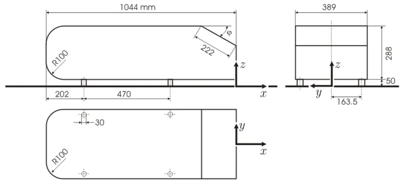
it looks similar to a car shape and once the numerical model is validated on this model we can uses that numerical model to design new car models.

the flow model for this simulation is turbulent, which is based due to the reynolds number that can be determined by the body length and the inlet velocity. turbulent kinetic energy is solved in addition to the velocity field in this simulation. A well refined mesh should be use in order to capture the wake zones and the boundary layers of the model.

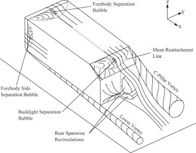
The three main characteric features that can be seen in this model are :

1. the recirculation region formed due to the flow seperation at the top of the vertical back surface of the wall
2. the recirculation region formed due to the flow seperation at the base of the model
3. the C-pillar vortices structure formed as the side boundary layer rolls up the slant rear edge of the model.

all the above discussed features can be seen in the following image

Importance of Ahmed Body:

The results from the experimentation over this model has shown that for slant angle less than `12^o` the flow remains attached to the surface , for slant angle `12^o < phi < 30^o ` there is a much of the 3 dimensional flow and C-pillar vortices are fromed at due to the rolling of the side boundary layer over the slant edge and results in increasing drag forces on the car body. at slant angle of `30^o` the strength of this vortices is maximum and thus has the maximum drag force. After this crtical value of the slant angle , the wake region reduce and so does the drag forces acting on the body. To achieve efficent vehicles with minimised fuel consuptions, CO2 emission and good driving stability this model is studied again and again to validate the results and design new car models .

Formation of Negative pressure :

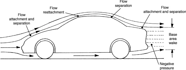
Wakes are the region of recirculating flow immediately behind a moving or stationay blunt body, they are genreally caused by the viscosity of the fluid. Wake are accompanied by flow seperations and turbulance.

In a fluid flow region over a body the viscous effects are ristricted to a thin layer known as boundary layer. the flow exerts a pressure force on the boundary layer. when the flow reaches the rear part of the ahmed body the fluid gets detached. Due to this there is a formation of large low pressure turbulent region at the rear end of the body ans the main cause for this negtive pressure is the viscous effects.

Significance of point of seperation:

Flow seperation is the detachment of a boundary layer from a surface into a wake. The flow seperation occurs when the flow slowss down and the pressure increases. this flow against increasing pressure gradient is known as flowing in an adverse pressure gradient . as the flow keeps flowing in an adverse pressure gradient after a limit the boundary layer stops or flows in the reverse direction this flow then becomes detached and the results into eddies and vortices. the fluid exerts constant pressure on the surface of the body once the flow is seperated. The flow seperation results in reduced lift and increased drag.

The seperation point is defined at the point where the wall shear stress is `tau underset(w)()` is equal to zero.

`((delu)/(dely))underset (w)() = 0`

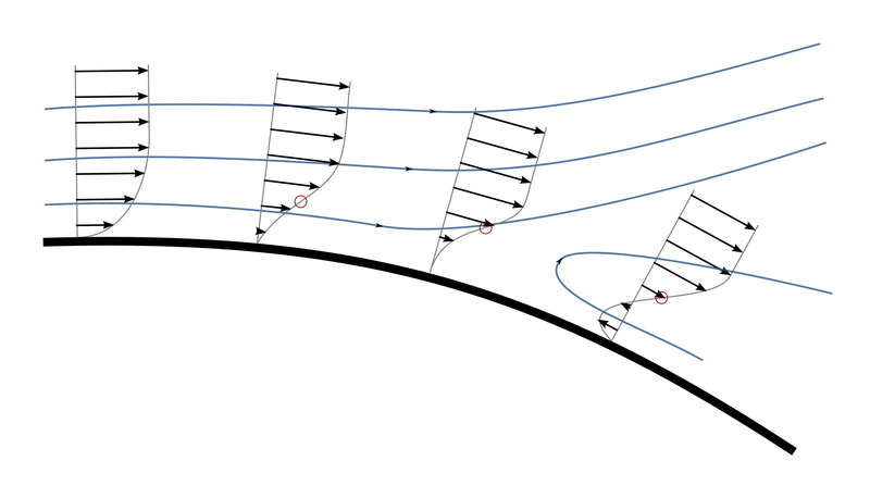
in the above image we can clearly see that as the flow through the adverse pressure gradient region the boundary layer is slowing down gradually and after certain time it reverses in direction. the point where the boundary layer velocity is zero is the seperation point.

Now we will be simulating for the external flow over ahmed body.

following steps are involved

1. improting the geometry into space claim and creating an enclosure around the ahmed body

2. create a baseline mesh to start with in the simulation process , later we will be refining the mesh to a smaller element sizing and perform grid independence upto the limit allowed by the software also keep the y+ value at the wall around 30.

3. setting up the fluent solution with k-epsilon model with standard wall function and set the inlet boundary conditions as 25 m/s .

4. We will run the calculation untill the drag and lift coefficient report definitions are stable and also the residual reach a stable state.

5. we will be observing the velocity and pressure contour and the vectors along the midplane and check for a detailed wake visiblity.

BASELINE MODEL:

the geometry was made by constructing an enclosure around the ahmed body and was splid in half to save the computation as the geometry is symmetric.

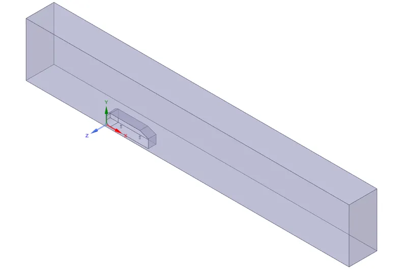
For the baseline simulation the mesh is the default that is generated by meshing and no meshing refinements were added . the mesh size is very coarse in this case. this simulation is for the understanding how the simulation works and what are the areas where we need to add more refinement can me observed . then in the next simulation we can add this improvisation to our mesh and capture results more correctly

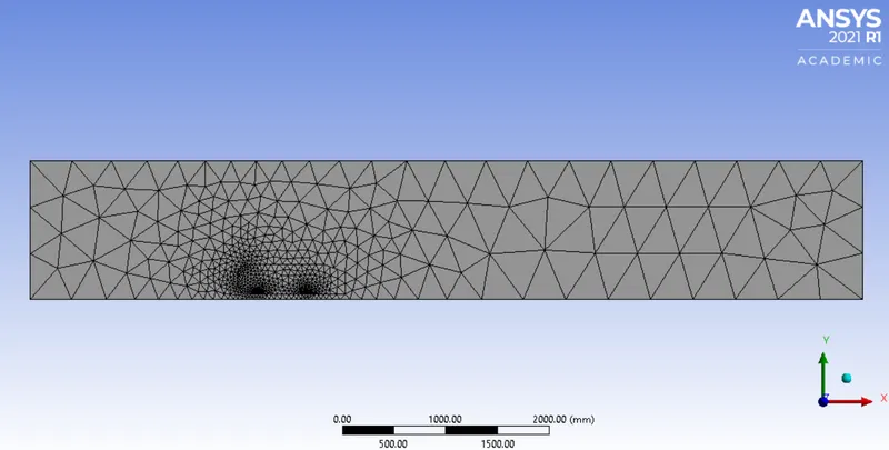
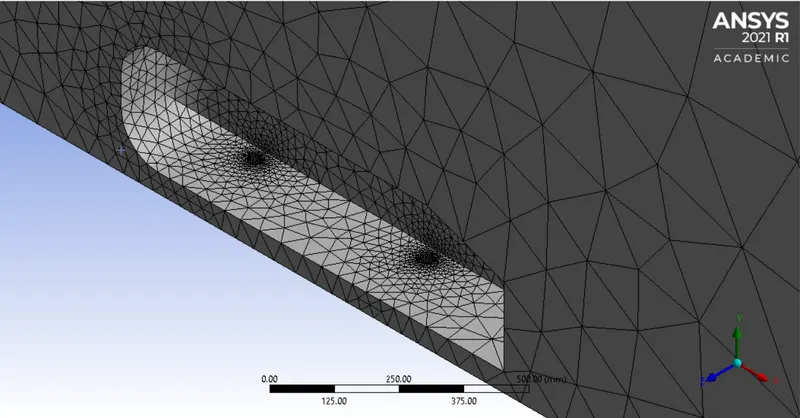
the details of mesh is shown below

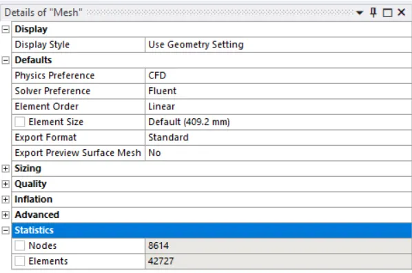
we can see that here the number of elements is 42727

the element quality metrics shows that the mesh is good quality

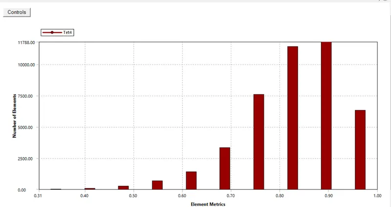
now this mesh is load into fluent.

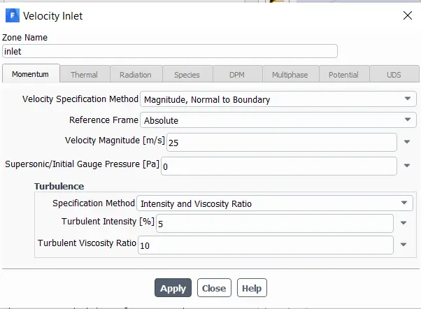
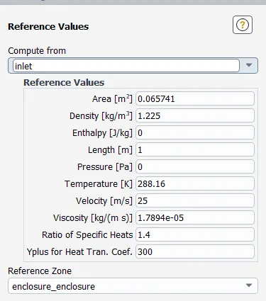
the fluent setup has the default air properties in this case and the inlet boundary condition was set to 25m/s . proper reference values were set according to the geometry and were computed from the inlet. the model was set to k epsilon turbulence with standard wall functions.

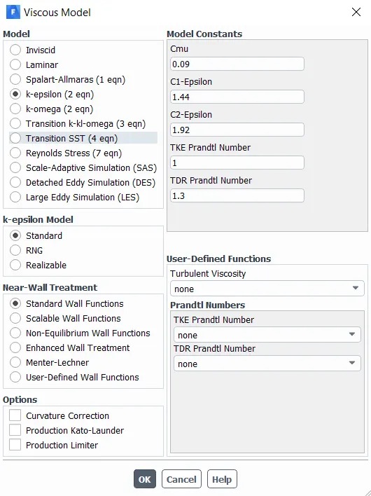
inlet velocity

reference values

we have run the simulation in a steady state upto 500 iteration so that the residuals and the reports definition reach a stable condition

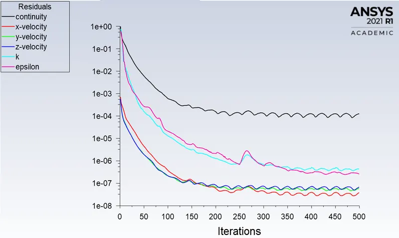
the residuals are fluctuating in the same range .

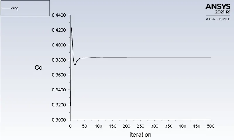
drag coefficient plot for iterations

lift coefficeint plot for iterations

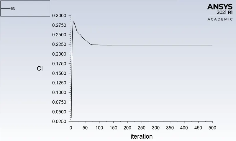
the lift and drag coefficients have been stavilized so our solution is converged

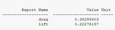
the lift and drag coefficeint values at the convergence are shown below

Now we will look at pressure and velocity contours

the pressure contour on the car wall is shown below

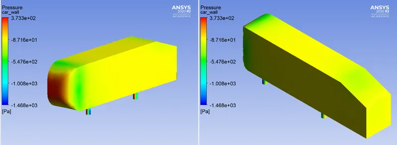
we can see that there is a high pressure region in the front of the car and then there is a low pressure region at the curve corneres in the front and the slant surface at the rear of the car .

the velocity contour si shown below

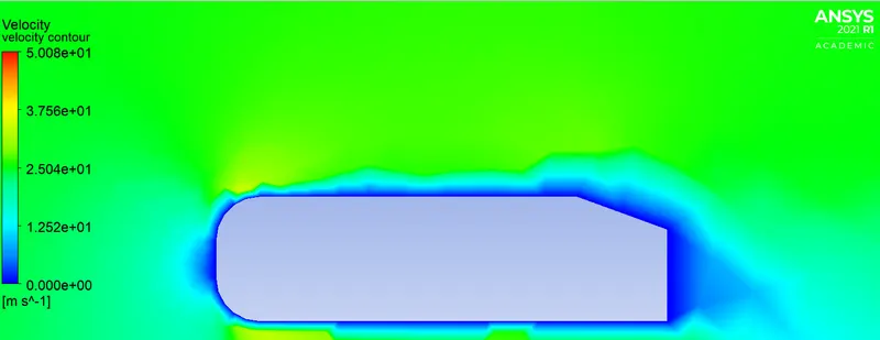
we can see the wake region forming at the rear end of the ahmed body but the wakes are diffusing due to the large mesh sizing.

now we know that we need to refine the wall boundary region and the wake region behind the body.

also we will look at the velocity vectors in the wake region

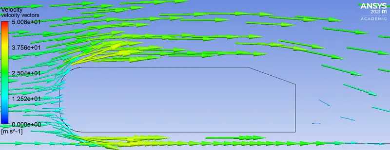
the vectors are not clear due to the coarse mesh

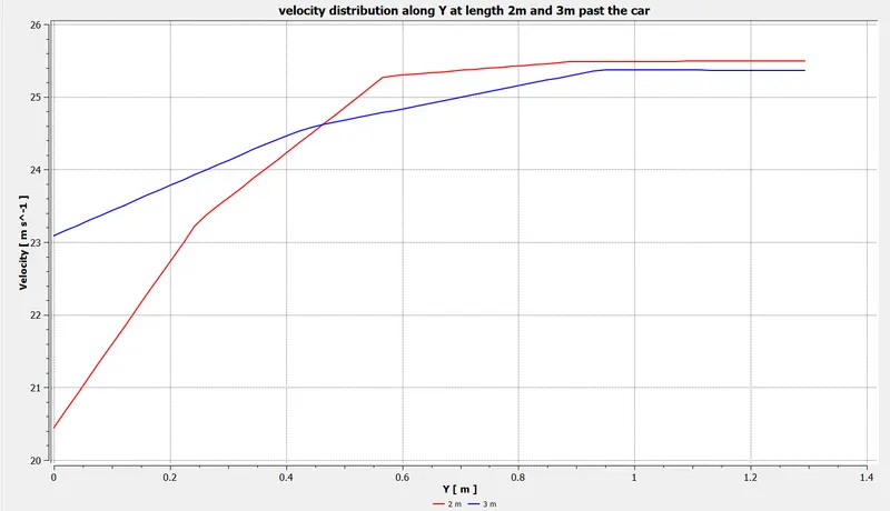
the velocity distribution along the y direction at length 2 m and 3 m at the rear of the car is shown below we can see the their are disturbance in the flow 3m past the car .

REFINEMENT 1:

Now we have refined our mesh using two enclosure so that our smaller enclosure can have refined mesh and the larger enclosure can have a mesh that is coarse and help save some computiation power.

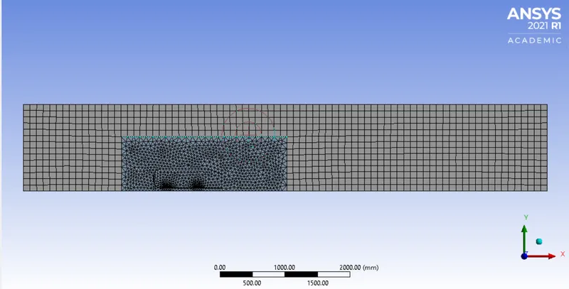
the larger enclosure has element sizing of 100 mm and the smaller enclosure has element sizing of 50 mm also we have added an inflation layer on the car wall of the first layer thickness of 0.429 mm to keep the yplus value 30. we have used 7 layer of inflation.

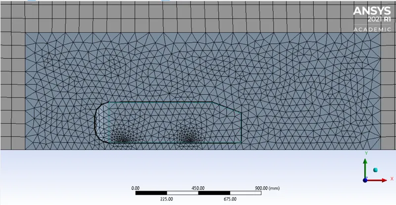
the number of elements in this model are

now this mesh was loaded in fluent and the simulation was run keeping all the parameter the exact same as for the baseline simulation. the results are discussed below

Residuals plot

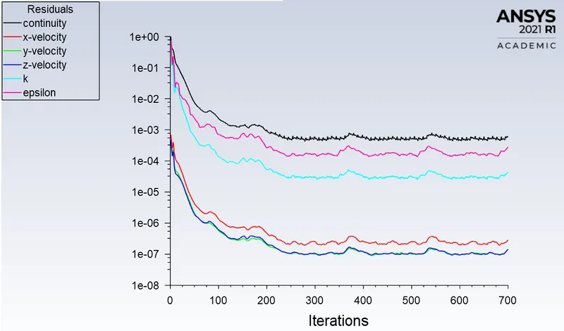the residuals are fluctuating in the same range

Drag coefficient plot

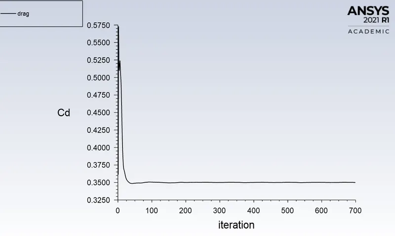
Lift coefficient plot

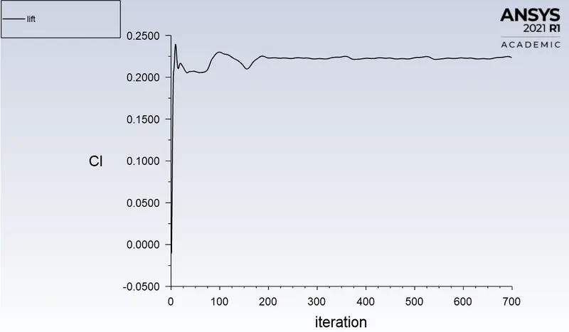
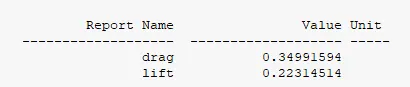
The drag and lift coefficients seems to have stabilised so our solution has converged at the followinf values of lift and drag coefficients

Now looking at the contour and vector plots for refinement 1

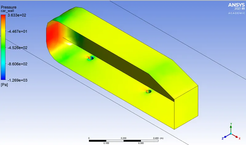
the pressure contour on the car wall can be seen and it has similar trend of pressure ar earlier

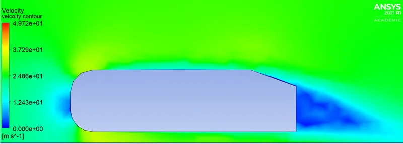
the velocity contour is showing a more refined wake region but though there are diffusions so the mesh needs to be refined more

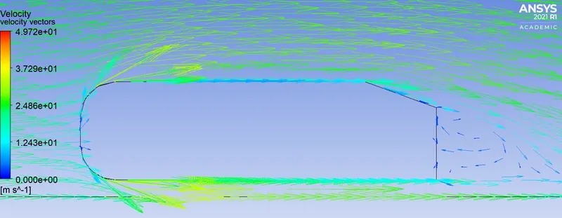
lastly the velocity vectors shows that the there is a recirculation zone in the wake region but the recirculations are not clear so more refinement is needed.

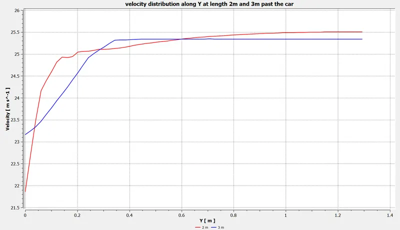
the velocity distribution along the y direction at length 2 m and 3 m at the rear of the car is shown below we can see the their are disturbance in the flow 3m past the car .

REFINEMENT 2:

In this case the element size in the smaller enclosure is reduced to 30 mm while keeing the external enclosure sizing at 100 mm.

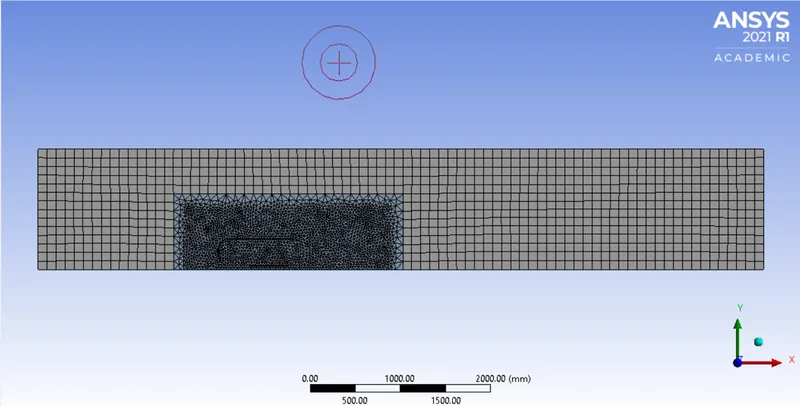
also an inflation was added of the same thickness as earlier to keep the yplus value at 30

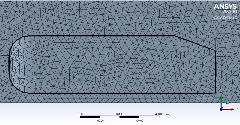
the mesh has a total 237557 elements

Now this mesh is used to run the fluent simulation and the results are discussed as below

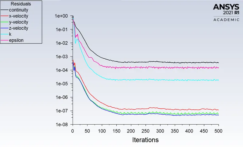
Residuals plot

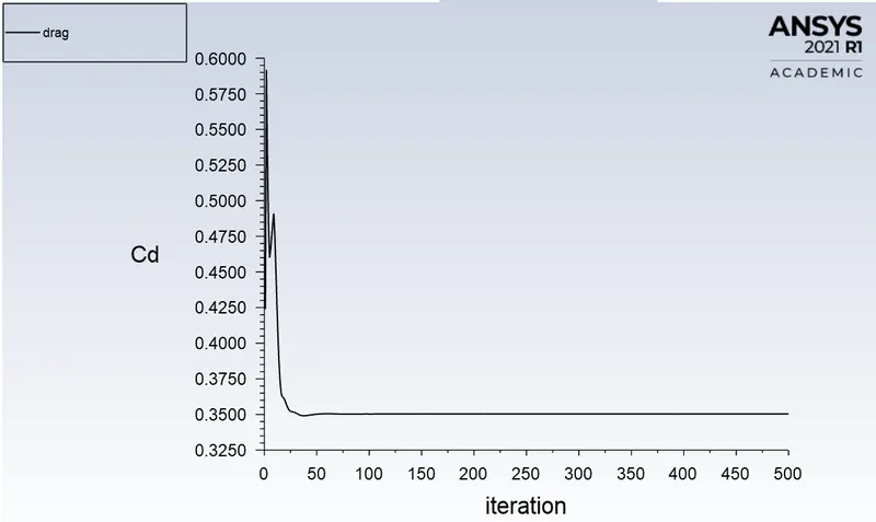
Drag Coefficient plot

Lift coefficient plot

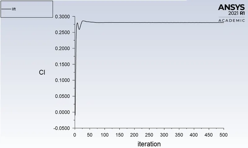
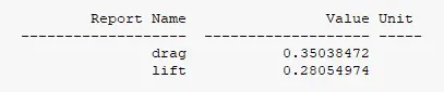
from the above plot it seems that the cefficients have stabilised so our solution is converged at the following values of lift and drag

the contour plot of the presusre and velocity are shown below

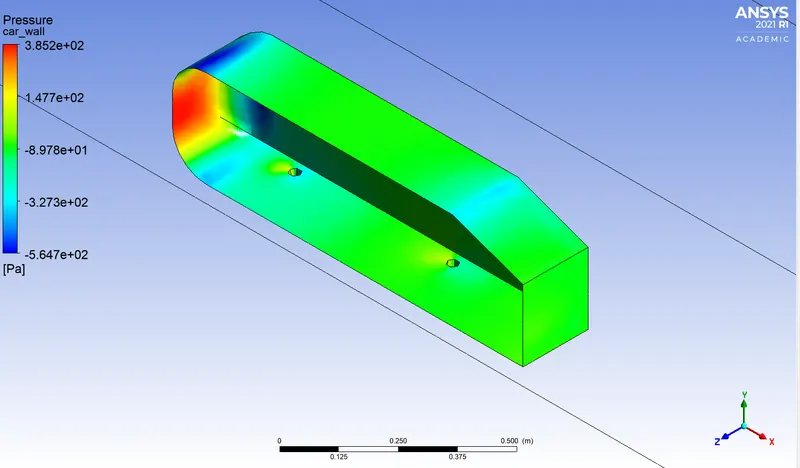the pressure at the wall is capture properly in this cases and the contours shows how the pressure is fluctuating along the car wall

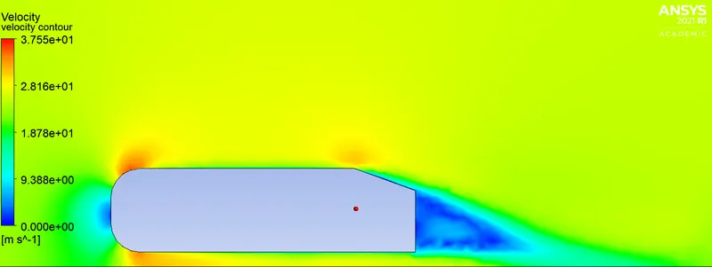
velocity contour

velocity vectors

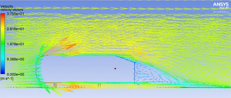
from the vector plot we can clearly see that there are two recirculation zones forming inside the wake region

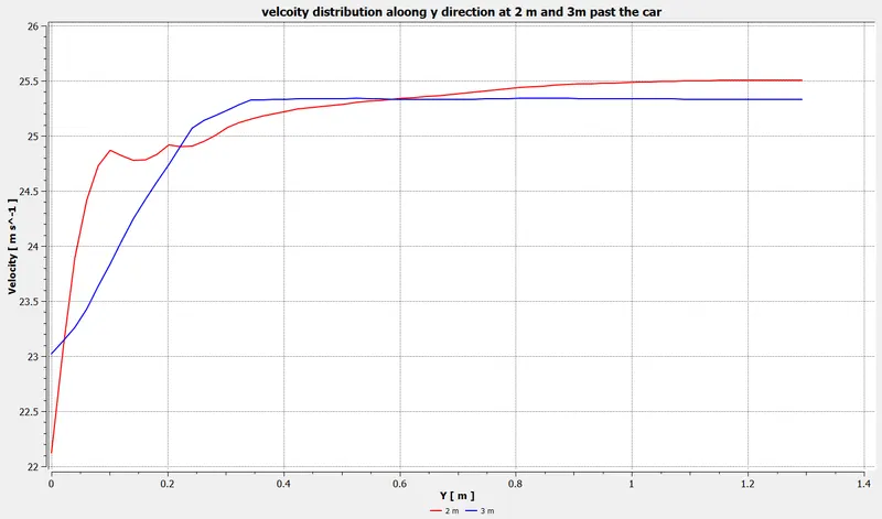
the velocity distribution along the y direction at length 2 m and 3 m at the rear of the car is shown below we can see the their are disturbance in the flow 3m past the car .

REFINEMENT 3:

In this case the smaller enclosure is kept at the element sizing of 25 mm and the outer enclosure is kept at 100 mm.

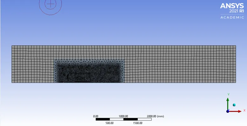
also same inflation setting we provided in this case as earlier

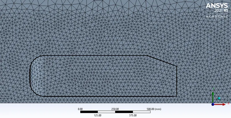
the total number of elements was 422942.

the results for the simulation using this mesh is given below

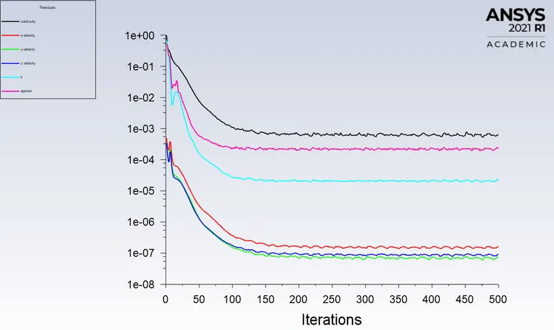
Residuals

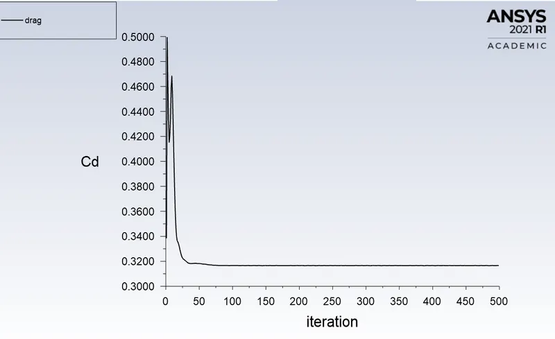
Drag coefficient plot

Lift coefficient plot

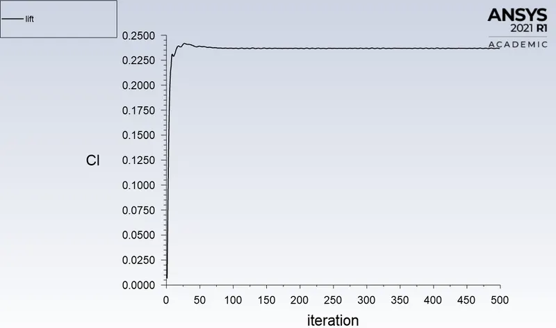
From the above plot it seems like our solution is converged as the report definitions of lif and drag have stabilized and also the residuals are flutiuating in a same range .

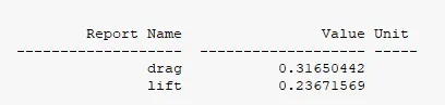
lift and drag coefficient values at convergence

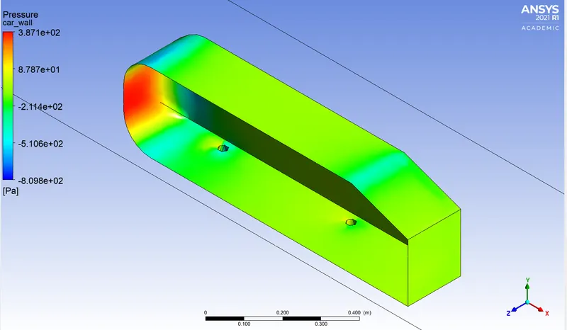
Pressure Contour

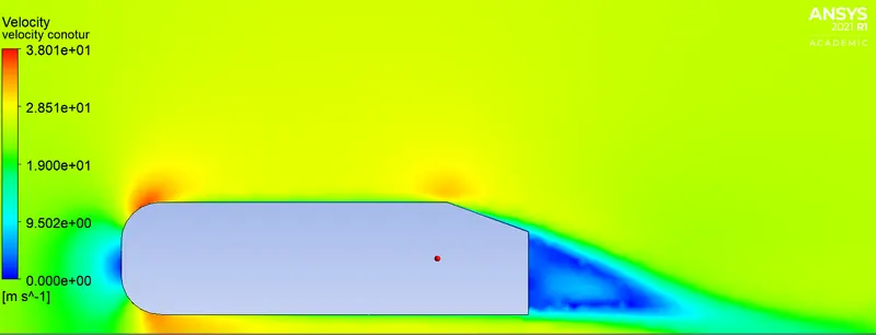
velocity contour

vecloicty vectors

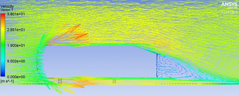
from the above vector and contour plots the results for the external fllow over ahmed body have good representation of the flow characterstics and the wake region is also clearly captured .

the velocity distribution along the y direction at length 2 m and 3 m at the rear of the car is shown below we can see the their are disturbance in the flow 3m past the car .

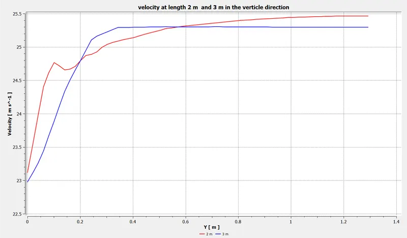
we could have refined the region in the wake but our acedemic fluent package restricts the simulation for that high number of elements. so we have to stop our grid independence test here itself.

We will be comparing the key parameters for various model used here in the following table

Parameters	Baseline Model	Refinement 1	Refinement 2	Refinement 3
elements size in the exernal enclosure(mm)	409	100	100	100
element size in the internal enclosure (mm)	-	50	30	25
Total number of elements genereated	42727	83621	237557	422942
first layer thickness of inflation	-	0.429	0.429	0.429
number of inflation layers	0	7	7	7y
y plus value	-	30	30	30
free stream inlet velocity(m/s)	25	25	25	25
Drag coefficient	0.3829	0.3499	0.3503	0.3165
Lift coefficient	0.2227	0.2231	0.2805	0.2367

The value of the drag coefficient is 0.31 for the most refined model.