External flow simulation over an Ahmed body

Aim:-

• Load the Ahmed body into Space Claim and split it into half as the body is perfectly symmetrical. Hence use symmetrical boundary conditions.
• Simulate the velocity of 25m/s with the default air properties in fluent.
• Describe Ahmed body and its importance.
• Explain the reason for the negative pressure in the wake region.
• Explain the significance of the point of separation
• Plot velocity and pressure contours over a plane.
• Plot the drag coefficient graph.
• Show the vector plot showing the wake region.
• Perform the grid independence test and provide the values of drag and lift with each case.

Objective:

• Study Ahmed body and its importance.
• Import the geometry in space claim, as the body is symmetric create symmetry fluid domain.
• Generate various mesh for the same geometry, to run the same simulation setup on each of the mesh which will tell us about mesh independence.
• Setup the mesh in fluent setup and simulate the velocity of 25 m/s with the fluent default air properties.
• Plot the drag and lift coefficient plot.
• Study the reason for negative pressure in the wake region.
• Also, study the significance of the point of separation.
• Post-process the results and plot velocity and pressure contour over a plane.
• Next, how the vector plot showing the wake region.
• Check the grid or mesh independence of all three cases.
• Finally, write a detailed report explaining all the processes, results, and plots.

Ahmed Body:-

The Ahmed Body was first created by S.R. Ahmed in his research “Some Salient Features of the Time-Averaged Ground Vehicle Wake” in 1984. Since then, it has become a benchmark for aerodynamic simulation tools.

The Ahmed body is a generic car body (a simplified vehicle model). The airflow around the Ahmed body captures the essential flow features around an automobile and was first defined and characterized in the experimental work of Ahmed. Although it has a very simple shape, Ahmed body allows us to capture characteristic features that are relevant to bodies in the automobile industry.

The simple geometrical shape has a length of 1.044 meters, a height of 0.288 meters, and a width of 0.389 meters. It also has 0.5-meter cylindrical legs attached to the bottom of the body and the rear surface has a slant that falls off at 20 degrees.

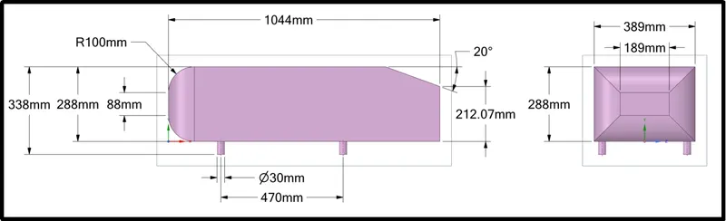
Importance of Ahmed body:-

As the burning of fossil fuels becomes a more pressing issue, manufacturers are introducing more fuel-efficient cars to the market. One main contributor to fuel burn is the car’s aerodynamic drag. Complexly shaped, cars are very challenging to model and it’s difficult to quantify the aerodynamic drag computationally. The Ahmed body is a benchmark model widely used in the automotive industry for validating simulation tools. The Ahmed body shape is simple enough to model while maintaining car-like geometry features.

This model is also used to describe the turbulent flow field around a car-like geometry. Once the numerical model is validated, it is used to design new models of the car.

Project setup

In this project we are going to set up the project in three case studies: In the first case study, we are going to use tetrahedral mesh all over the fluid domain with fine meshing near the car body wall and coarse mesh at the other area.

In the second case study, we are going to create separate fluid volumes for fine tetrahedral mesh near the car surface, and for another volume, we are going to use hexahedron mesh.

In the final case study, we are going to make the mesh a little finer and also increase the number of inflation layers.

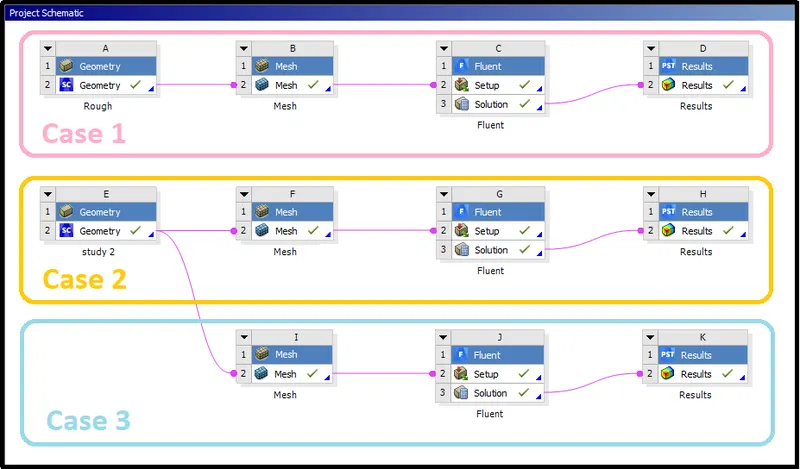
After setting and running all three setups, we will be going to compare the results to check the mesh dependency of the setup.

Preprocessing

Case study setup 1

Prepare the geometry for meshing (CAD)

to start, let us import the geometry of Ahmed body in space claim. In CFD we need the fluid region and cavity of geometry for meshing and simulation. Therefore, we have to specify fluid and create a cavity of geometry in space claim.

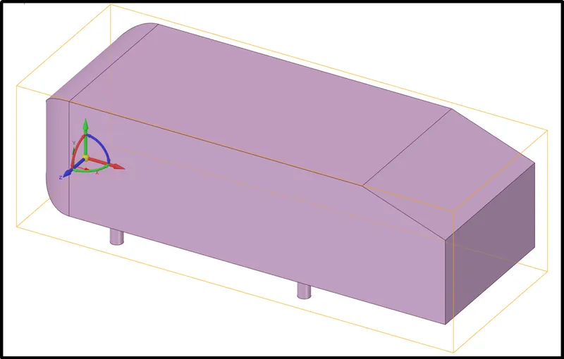
Firstly, load the Ahmed body into Space Claim which will represent the part in Space Claim Graphical user interface as shown in the below figure.

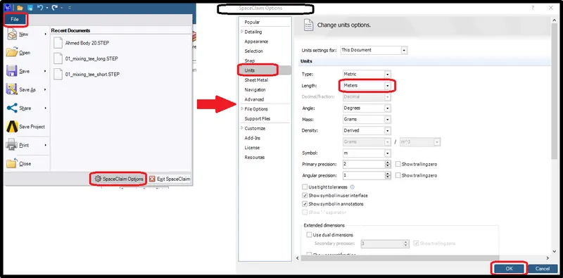
Default units in Space Claim will be in mm to convert it go to File -> click on SpaceClaimOption button -> unit -> change length into the meter and click OK.

The next step is to create the fluid region with the cavity of loaded CAD geometry. To do that go to Prepare -> select Enclosure.

It will create the enclosure around geometry with user-defined dimensions. We are using the dimension as shown in the following figure.

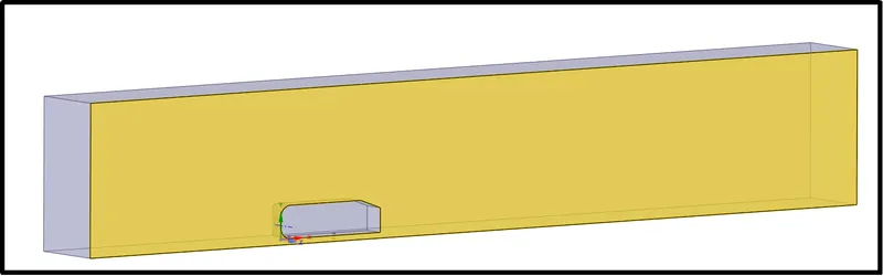
The above process creates an enclosure around the Ahmed body as shown in the below figure. As the body is perfectly symmetric about the X-Y plane we can split it into half.

Splitting will let us use fine mesh with half of the number of cell grids(mesh). Also, as it uses half the number of elements it will save our computational time.

So, create the plane with the reference of the axis system of the loaded geometry. Go to design -> select icon of plane -> click on the axis on the geometry. It will create the three planes as exhibited in the below figure.

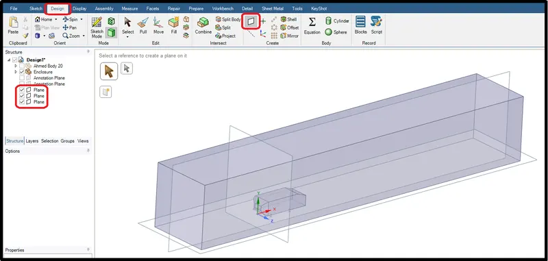
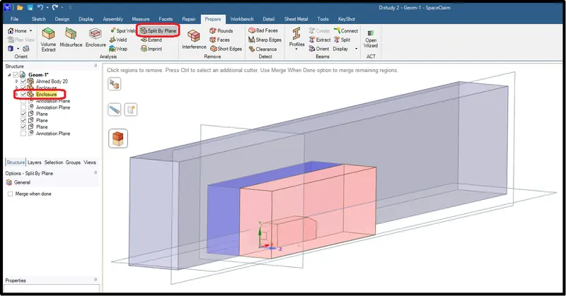
To split the enclosure body, go to -> Prepare -> click on Split By Plane. After that, select the plate by which the body required to be split and select the side required to be removed.

After, splitting the body symmetry half section will look as shown in the below picture.

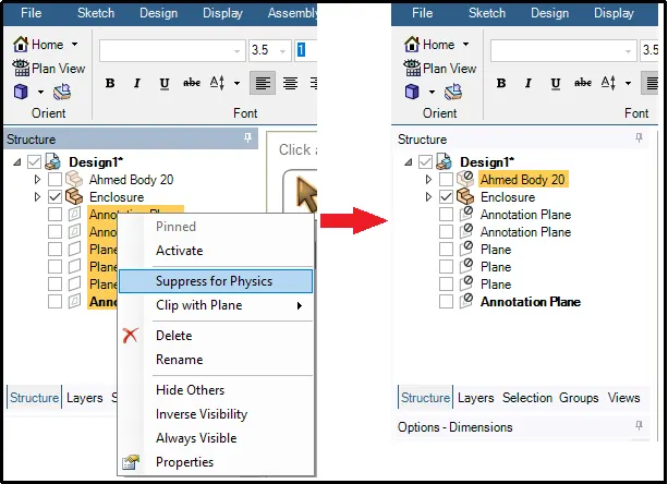
Now, our geometry is ready for the case1 study. Keep the required enclosure part and suppress all the remaining entities.

Meshing (Case 1)

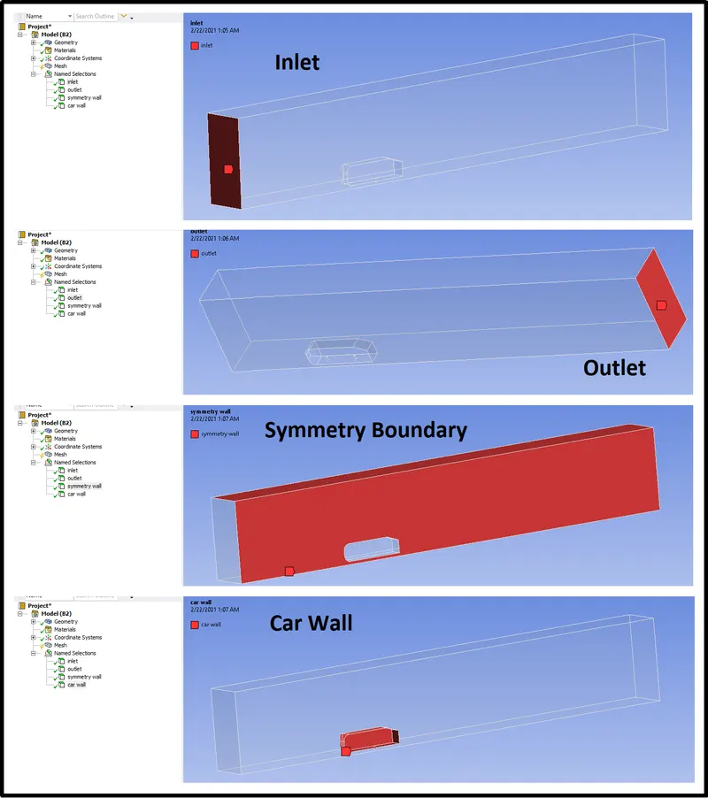
Next, open the meshing module where we will provide the name to the surfaces of the fluid domain and mesh it.

Apart from the inlet and outlet name, to the other surface, we are going to define as symmetry wall and car surface as car wall.

For meshing, mesh the domain as a tetrahedral dominant mesh with a regular and max size of element as 100mm.

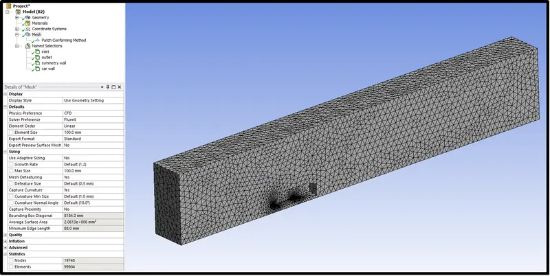
In this case study, we have to measure the parameters near the car surface. Therefore, we will need a very fine mesh near the car surface.

As we are using Ansys academic version, we have a limitation of cell grids, up to 51200 cells, so on the remaining area of the fluid domain, we are going to use coarse mesh. Hence, change element size value to 150mm and max element value to 200.

Add sizing to the car surface and use an element size of 20mm.

The holes have a diameter of 30mm so for hole surface it is better to use element sizing of 5mm. For overall geometry we will keep a growth factor of 1.2, meaning the mesh will increase to its normal size of 150mm by 20 percent with each element. After generating the mesh, we will get the following results.

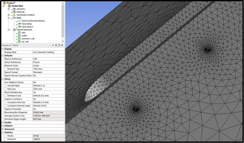
Finally, to capture surface boundary results accurately we need a fine inflation layer over the car wall. In a bid to find out first layer thickness Y-Plus boundary layer estimation is vital.

Y+ Boundary layer

The behavior of the flow near the wall is a complicated phenomenon and to distinguish the different regions near the wall the concept of wall Y+ has been formulated. Thus Y+ is a dimensionless quantity and is the distance from the wall measure in terms of viscous length.

In the turbulent boundary layer region flow near the wall has been analyzed in terms of three layers.

• The inner layer, or sublayer, where viscous shear dominates.
• The outer layer, or defect layer, where large-scale turbulence eddy shear dominates.
• The overlapping layer, or log layer where velocity profiles exhibit a logarithmic variation

One of the reasons for the need for Y+ is to distinguish different regions near the wall or in the viscous region, however, how exactly it helps in turbulence modeling or in general CFD modeling need to be well understood. If we intend to resolve the effects near the wall i.e., in the viscous sublayer then the size of the mesh size should be small and dense enough near the wall so that almost all the effects are captured. But in some cases, if the wall effects are negligible then there is the option of including semi-empirical formulae to bridge between the viscosity-affected region and fully turbulent region, and in this case, the mesh need not be dense or small near the wall i.e, the coarse mesh would work.

Considering the first case, i.e., near-wall modeling it is well-known that the mesh size should be small enough, however then the question following is how small? Thus, here comes the concept of Y+, and based on the Y+ value the first cell height can be calculated. The near the wall region is meshed using the calculated First Cell height value with gradual growth in the mesh so that the effects are captured and avoiding overall heavy mesh count.

Calculating the first Cell Height for a desired Y+ value

Firstly, we should calculate the Reynolds number for our model based on the characteristic scale of our geometry such that:

`Re = (rho.U.L)/mu`

Where,

`rho` is the fluid density

`mu` is the viscosity

U is the free-stream velocity,

L is the characteristic length

So, free stream velocity = 25m/s, Density = 1.225kg/`m^3`, Dynamic Viscosity = 1.7894e-05kg/ms, Length = 1.044m

`Re = (1.225xx25xx1.004)/(1.7894e-5)`

`Re = 1.79xx1e-5`

The definition of the Y+ value is such that:

`Y+ = (rho.U_tau.Deltay_1)/mu --> Delta y = (Y+.mu)/(rho.U_tau)`

The wall shear stress, `tau_w` can be calculated from skin friction coefficient, `C_f`, such that:

`tau_w = 1/2. C_f.rho.U^2`

The ambiguity in calculating DeltaY1 surrounds the value for `C_1`. Empirical results have been used to provide an estimate to this value:

For internal Flow type --> Empirical Estimate (`C_f = 0.079. Re^-0.25`)

For External Flow type --> Empirical Estimate (`C_f = 0.058. Re^-0.2`)

Use `C_f` for external flow,

`C_f = 0.058 xx (1.7862e+06)^-0.2 = 0.0033`

`tau_w = 1/2(C_f)(rho)(u^2)`

`tau_w = 1/2(0.0033)(1.225)(25^2)`

`tau_w = 1.2475`

Friction velocity

`U_f = (tau_w/rho)^0.5`

`U_f = (1.2475/1.225)^0.5`

`U_f = 1.0091`

Mach number

`Mach N u mber = U/340 = 0.0735`

For Y+ = 30 first layer thickness

`Delta y = (50xx1.7894e-05)/(1.225xx1.0091) = 0.00043426856m`

For Y+ = 40 first layer thickness

`Delta y = (50xx1.7894e-05)/(1.225xx1.0091) = 0.00057902475m`

For Y+ = 50 first layer thickness

`Delta y = (50xx1.7894e-05)/(1.225xx1.0091) = 0.00072378094m`

now, in this case, we are considering Y+ 50 calculation. If we do not obtain the desired thickness, then we do it by hit and trial way.

Number of layers

n = 15

Growth rate

Gr = 1.2;

Total thickness

`T_t = Delta y *Gr^(n-1)`

`T_t = 9.2956 ~ 9`

We can then input these known values into the above equation to estimate our value for `Delta y`.

When considering simple flows and simple geometry, we might find this correction is highly accurate. However, when considering complex geometry, refinement in the boundary layer may be required to ensure the desired Y+ value is achieved. In these cases, we can choose to re-mesh in Ansys meshing to use anisotropic mesh adaption (i.e. Adaption of local cells only in the wall-normal direction) to achieve your desired Y+ value across the entire model.

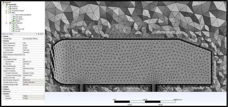
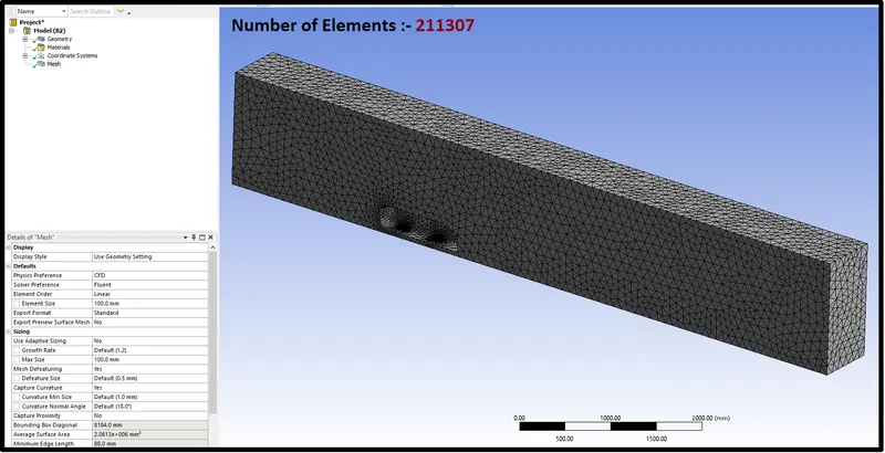
Our final cell count will be 211307 which is less than the minimum criteria of cell count in the academic version.

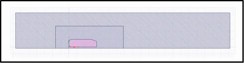
Case study setup 2

For case 2 setup, we are going to create a separate volume near the car wall, this volume dimension can only be guessed after running the simulation on a coarse mesh and studying the behavior of the fluid mesh.

By using the following dimension we are going to create a new enclosure near the car surface.

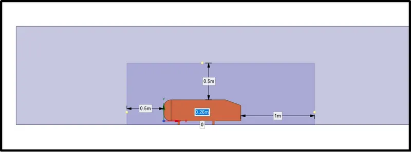
Same way, using the split by Plane button split this volume too. Now, we will be able to see there are two enclosures created in the structure tree.

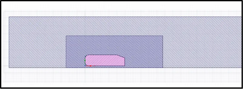
But if we cut them into sections, we can notice that the two volumes are overlapped with each other.

To verify it properly, use the ‘interference’ button in prepare section. It will highlight the volume that interfaced with each other in red color. Just by clicking green right-click, we can solve this problem.

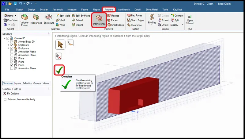
Now, we can see that there no interference in the two volumes.

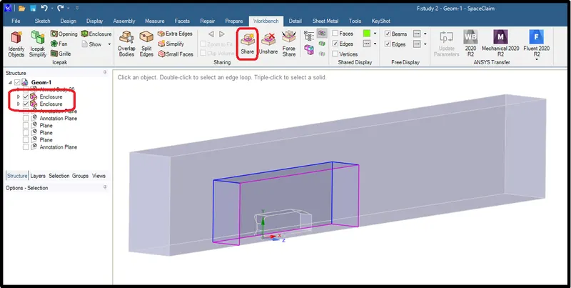
Lastly, before closing the Space claim share the two-volume (Enclosure), otherwise, fluent will treat it as a different body.

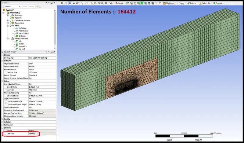
Meshing (Case 2):

In case 2, we will execute hexahedral meshing on the outer volume and fine tetrahedral meshing on the inner volume

We will provide a small element size of 20mm on the car wall and 8mm near holes with a growth rate of 1.2.

Finally, to capture the proper viscus and drag effect near the car wall, we are going to use the inflation layer same as we used in the previous case.

Case study 3

Geometry :

In case study 3 we are going to use the same geometry setup as we used in case 2

Meshing (Case 3):

In the meshing of case study 3, we are going to refine the mesh size of the car wall and increase the inflation layer.

Inflation layer calculation.

For Y+ = 50 first layer thickness

`Delta y = (50xx1.7894e-05)/(1.225xx1.0091) = 0.00072378094m`

Number of layers

n = 20

Growth rate

Gr = 1.2;

Total thickness

`T_t = Delta y *Gr^(n-1)`

`T_t = 23.1304 ~ 23`

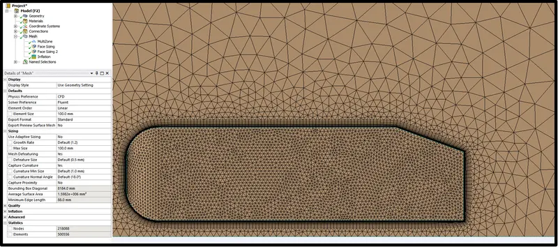
Here, for car walls, mesh sizes are 10mm and 5mm at holes with a growth factor of 1.2.

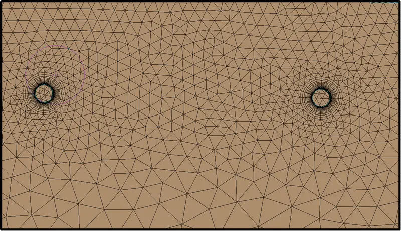
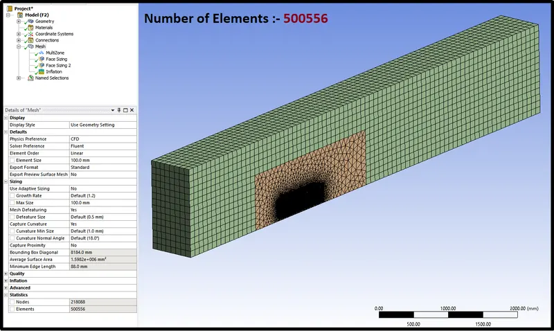
Fluent setup

After meshing our fluent setup for all three cases will be identical.

Open fluent setup, we will first check mesh. Then we set up a general setting

General setup

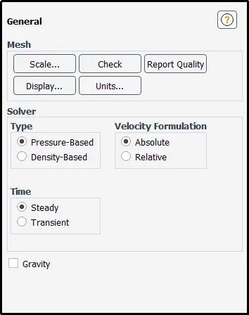
Then we will set the physics of the domain. Keep the general parameter setting as it is. Solver type -> pressure-based; velocity formulation -> Absolute; solver time -> steady.

Solver type

In this case, mach number is 0.0735, which is less than 0.3, hence we have to use a pressure base solver. In case the mach number is greater than 0.3 we will have to use a density-based solver.

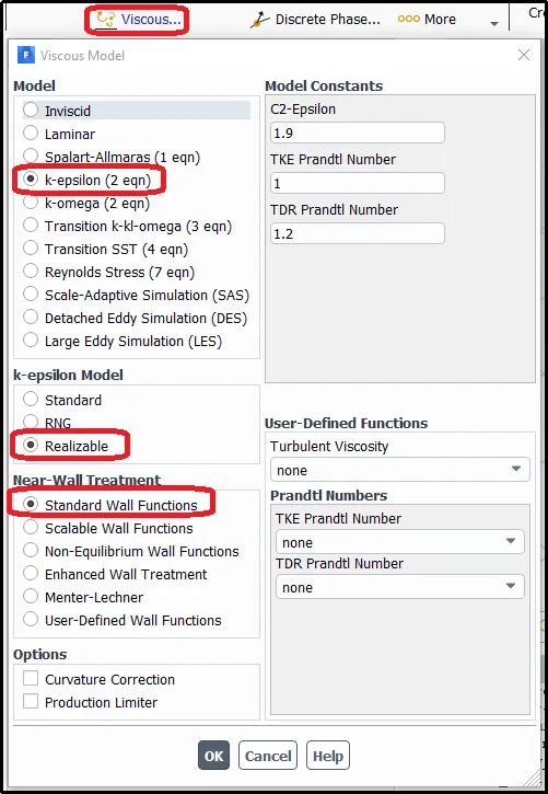
In the viscus model, select ‘k-epsilon’,’ Realizable’ for our first type of simulation. Turbulence modeling is a complex area. The choice of model depends on the application. Here, the Realizable k-epsilon model is used which is an improvement on the well-established standard k-epsilon model. Accept the remaining default settings.

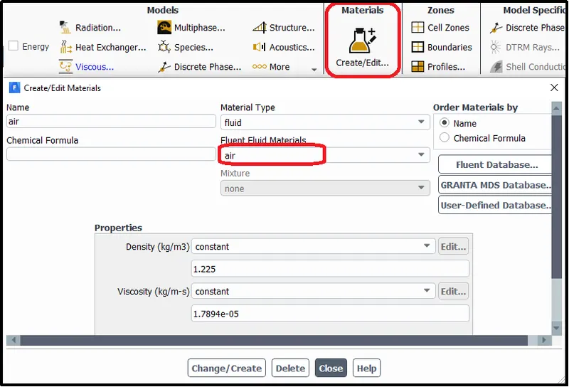
Fluid Material we are going to use air which is a default material of the fluent

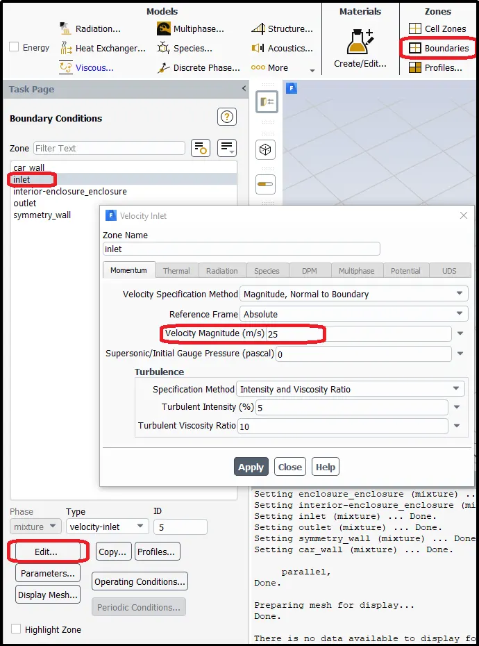
Air will flow with the inlet velocity of 25m/s.

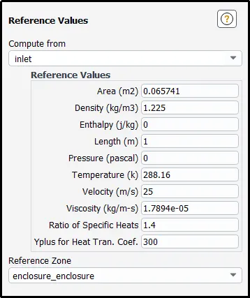
Reference Values:

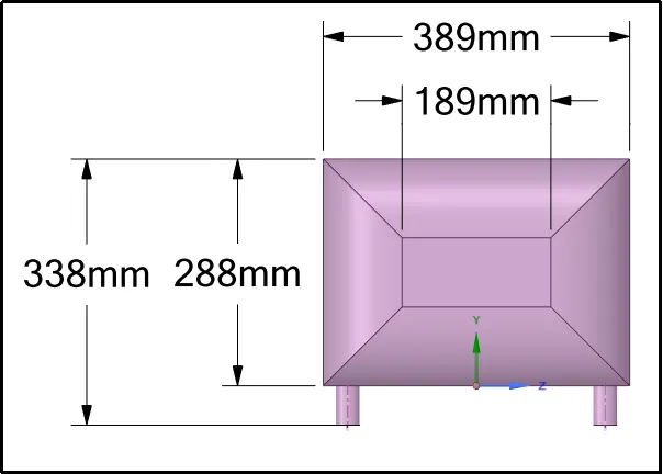
`Area = 0.338xx(0.389/2) = 0.065741m`

Initialization

In initialization, we are going to use a hybrid initialization method.

The hybrid Initialization method is an efficient method of initializing the solution based purely on the setup of the simulation with no extra information required. These methods produce a velocity field that conforms to complex domain geometries and a pressure field that conforms to complex domain geometries and a pressure field that smoothly connects high and low-pressure values.

Now, we can run the simulation just enter several iterations for which we want to run the simulation and press ‘calculate’.

Results

Residual plot:-

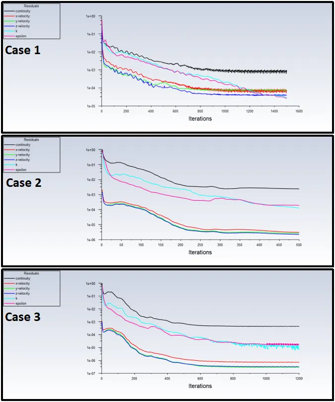
In the residual plot, for complete tetrahedral mesh, we see a lot of fluctuation in results. In contrast, other two study shows smooth convergence. But in the last case, we see little fluctuation in convergence after 800 iterations. But we can say these results are converged because besides small fluctuation it's not showing any other changes.

Drag Coefficient

Drag Coefficient in cars

The drag coefficient quantifies the resistance of an object in a fluid environment. It is not an absolute constant for a body’s shape because it varies with the speed and condition of flow, abject shape and size, and the density and viscosity of the fluid. The lower the drag coefficient of an object, the less aerodynamic or hydrodynamic drag occurs. In terms of a car, the lower the drag coefficient, the more efficient the car is. As well as affecting the top speed of a vehicle, the drag coefficient also affects the handling. Cars with a low drag coefficient are sought after, but decrease the drag drastically can reduce the down-force and lead to a loss in road traction and a higher chance of car accident.

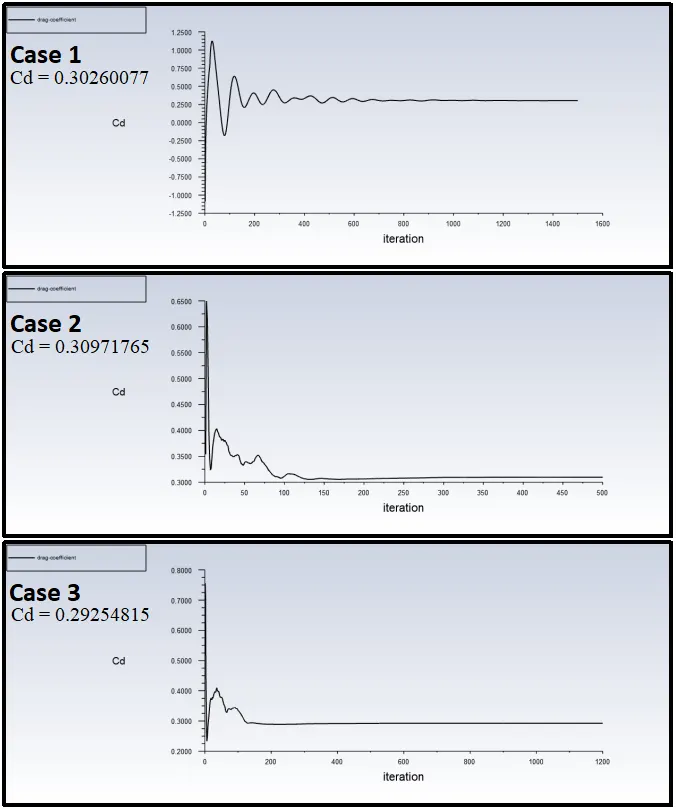
The above figure represents the drag coefficient graph for Ahmed body at a velocity of 25 m/s. we can see as the mesh getting finer we are getting our results more early.

Lift Coefficient

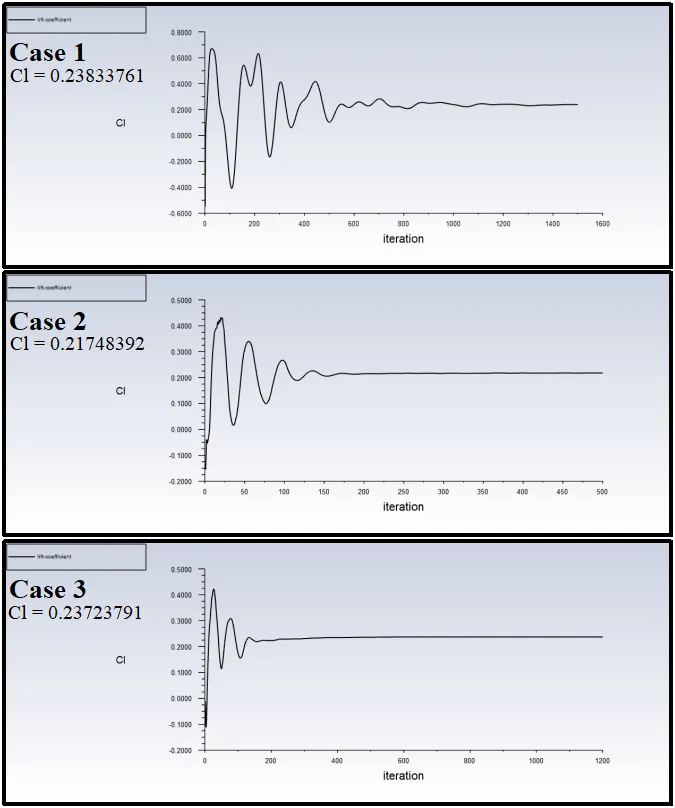
As shown in the figure, we get to know that like drag we are getting our result to converge earlier as we are making mesh finer. The fluctuation in results also reducing accordingly.

Pressure contour over the plane, plane along two holes and over a car body

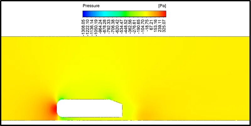
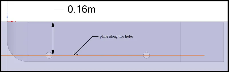
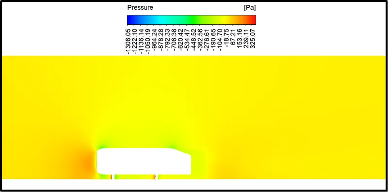
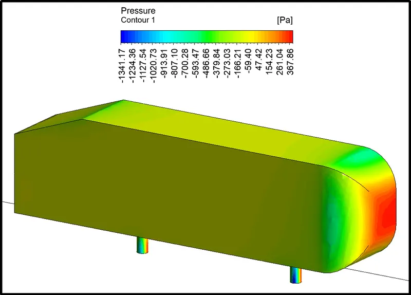
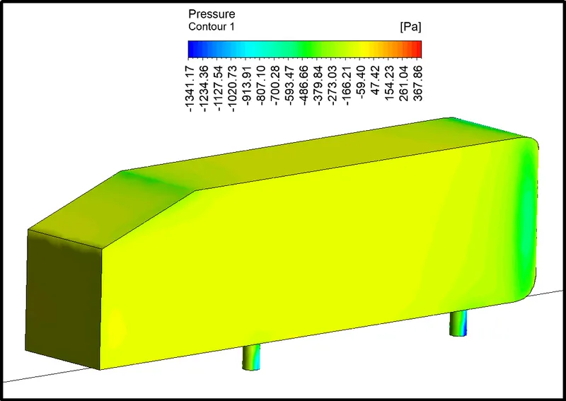
The above pictures exhibit the pressure distribution over the can body and how pressure behaves with the flow over an Ahmed body.
One thing we can notice, it shows the negative pressure over a body from the weak region.

Negative pressure in the wake region:-

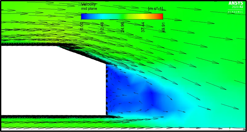
The wake region is a distributed flow region or usually turbulent flow around a solid body moving through a fluid. This phenomenon is mostly caused due to the boundary layer separation which creates a high turbulent flow zone. This separation is caused by the adverse pressure gradient (High-pressure drops) giving a net pressure force. The velocity and pressure in this region are low and increase the drag force on the body. Since the drag force also depends on the wake region, the Formulation of the wake region is one of the important characteristics to consider while designing an automobile.

The negative pressure in the Ahmed body is due to bluff bodies. The boundary separation and recirculating of the flow and also the effect of shear stress. To overcome the shear, stress pressure turns negative to balance the effect.

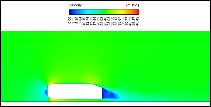
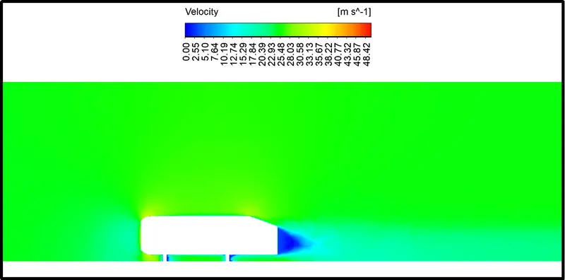
Velocity Plot over a midplane and plane along two holes

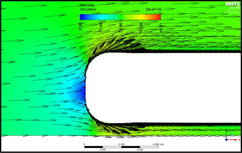
Streamline flow and vector plot

Significance of the point of separation:-

The point of separation is a point where the fluid flow no longer follows the contour of the body and gets detached from the surface of the body. When there is a fluid flow over a solid body there a retarding effect on the fluid flow that detaches from the surface giving rise to vortices and Eddie forces. Once the fluid is detached it exerts constant pressure on the surface instead of exerting a continually increasing pressure.

The boundary separation and recirculating of the flow and also the effect of shear stress. To overcome the shear, stress pressure turns negative to balance the effect.

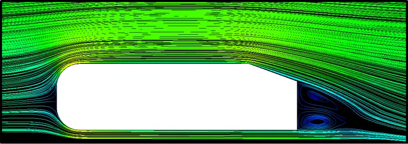
The wake region increased the thrust force caused by the body depicted in the vector plot and the drag which extends behind the body. This makes the back-flow which travels from high to lower pressure region and the vortex is formed.

Velocity monitor at various distance from inlet wall

to observe velocity changes at the various locations from the inlet we are going to create a few monitor probes (lines) which will give us the data about velocity along the y-axis at the mid-plane.

The velocity plot of all the cases are almost similar to one another so following are the results of fine mesh (Case 3).

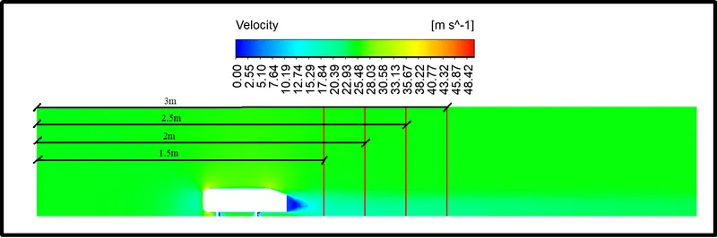
Velocity monitor plot at various distance from the inlet

• Series 1 - at distance 1.5m
• Series 2 - at distance 2m
• Series 3 - at distance 2.5m
• Series 4 - at distance 3m

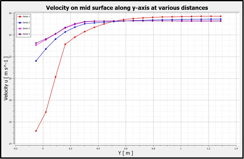
Velocity monitor reading at various distance from the inlet

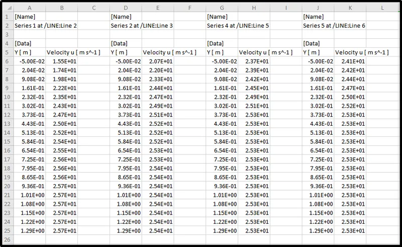
Mesh Dependency:-

In the overall project, we perform the simulation three times with the different numbers of elements to verify that converged results are not varying because of grid (mesh) size.

The above table shows the values of drag and lifts coefficients for different no of elements and various grid sizes. Differences in both the values for each mesh are very less, which means results are considerable.

Conclusion:-

• When the geometry is symmetrical in nature we can use its section symmetrical part, which can help us to the drastic reduction in mesh grid elements lead to minimizing computational time and power.
• Ahmed body can use as a dummy simulation to set the setup for other car bodies. By doing this, we can verify our results which got from rough simulation to validate our simulation setup for actual geometries.
• Generating mesh with the reference of Y+ value improves the accuracy of results at the surface when the flow is turbulent near the wall faces. It also affects the accuracy of drag and lift coefficient values as this value we observe at the wall surface.
• The negative pressure around the body is generated due to the boundary layer separation which creates a high turbulent flow zone.
• The boundary separation and recirculating of the flow and also the effect of shear stress. To overcome the shear, stress pressure turns negative to balance the effect.
• A grid independence test is important to validate the generated mesh of the final setup.

References:-

[1] Flow and Turbulence Structure in the Wake of a Simple Car Model -https://www.researchgate.net/publication/266883948_Flow_and_Turbulence_Structures_in_the_Wake_of_a_Simplified_Car_Model_Ahmed_Model

[2] Experiments and numerical simulations on the aerodynamics of the Ahmed body -https://www.researchgate.net/publication/330383775_Experiments_and_numerical_simulations_on_the_aerodynamics_of_the_Ahmed_body

[3] Basics of Y Plus, Boundary Layer and Wall Function in Turbulent Flows - https://www.learncax.com/knowledge-base/blog/by-category/cfd/basics-of-y-plus-boundary-layer-and-wall-function-in-turbulent-flows

[4] Aerodynamic drag reduction and flow control of Ahmed body with flaps - https://journals.sagepub.com/doi/full/10.1177/1687814017711390

[5] Effect of slang angle variation on the drag force for Ahmed body car model - https://www.jvejournals.com/article/21115