Project Report

Introduction

Ahmad Body (car model) is a simplified vehicle model concept, primarily used in studying the aerodynamics of vehicle. The length of the model stands out to be 1.044m, the width is of 0.389m and height stands to be around 0.288m. It has 4 pillars for simulating wheels, the diameter of which is 30mm and height of 50mm. It also has a slant surface on its back, its angle can be changed to study the effect of drag on varying geometry.

Like every simulation has huge benefit of cost reduction before the real experiment, the car model discussed above also servs the same purpose. The model works as a generic vehicle, it has all the features from the aerodynamic point of view. So it has great importance in studying force that surrounds the vehicle and in turn affects the fuel consumption.

Objective

To carry out grid independence study with an aim of calculating drag and lift coefficient.

Modelling

In order to achieve the objective of the study, work is progressed by making a baseline mesh at first. Then it has been further improved till the constrain of the computational power available.

Since we are interested in drag and lift calculations, we need a nice approach to model our boundary layer phenomenon.

In order to have a decent approximation of those coefficients, Y+ has a big role to play. For the present study Y+ of 30 has been choosen.

Calculation of the first cell height based on y+

`Re = {rho*U*L}/{mu}`

where, Re is the renolds no.

U, L are the free stream velocity and characteristics length respectively.

`mu` is the viscosity.

As per our simulation case,

Re when calculated is, `1.78 X 10^6`

Calculation if skin friction

`C_f`= 0.058 x (1.78 * 10^6)^{-0.2} = 0.0033

`tau_w` = 1.2475

`U_f = ({tau_w}/{rho})^0.5` = 1.0091

for Y+ of 30

first layer thickness = `{y_+ * nu}/{rho*U_t}` = `4*10^-4`m

Though we have calculated, first layer thickness based on the constrains of computational power, we will go for first cell height of 0.001m

Baseline Setup

Geometry

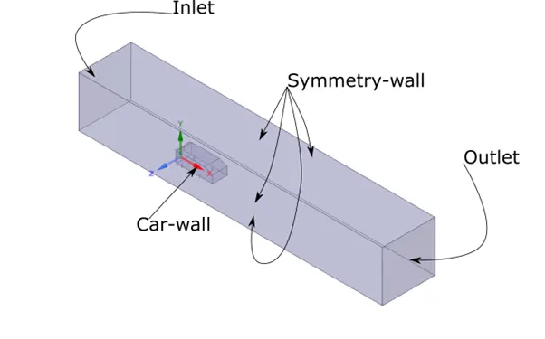
Ansys – SpaceClaim has been used to preprocess and setup the geometry for simulation. The given model contains the simulating geometry of car. We require to provide the computational domain for fluid around the main geometry for simulating the airflow. The same has been achieved by building an enclosure around the main model. The enclosure box begins 2m before the front of the car model, it continues 5m beyond the rear end of the model. Height of 1 m above the car model has been given to the enclosure box.

Meshing

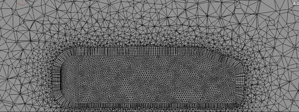
Built-in Ansys module for meshing was used to mesh the domain. The default size of the elements was restricted to be of 0.1m. Various other sizing constraints are applied in vicinity of the car model.

Around the surface of the car body, element size of 0.01m were employed. Since the pillars has circular geometry, so the element size was reduced to 0.001m around the 4 pillars.

A five Layered inflation with initial height of 0.01m was employed around the car body for viscous flow modelling.

Solver

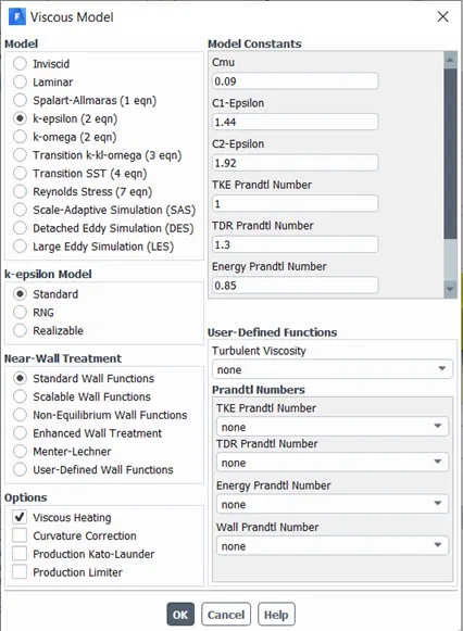
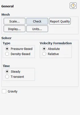
Ansys Fluent has been used to solve the present computational model. Since the Mach No. is less than 0.3, pressure-based solver has been employed for the same. Standard K-epsilon method has been employed as the viscous model. Steady State solution has been computed for the present case.

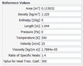
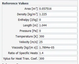
For Ansys module to calculate drag and lift coefficients, reference value of area was set as that of cross-section obstructing the flow, i.e., 0.115032m2. The length was set to 1.044m.

Boundary Conditions

Inlet

Inlet has the velocity input boundary condition with a magnitude of 25 m/s.

The outlet has zero-gauge pressure, The symmetry wall has symmetry boundary condition.

Scope for better analysis

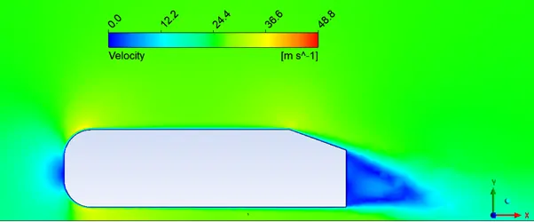
Running the base line simulation gives the idea of computational complex zones in the present model. In order to refine the study further, various modification has been done. In order to get a better idea of the refinement zones, the vector and contour plot has been made as below.

Contour Plots

Velocity Contour Plot

Pressure Contour Plot

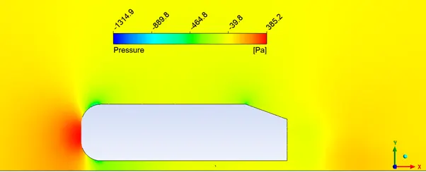
The contour plot shows the leading and trailing sides of the car model. The profile has lots of gradient that has been averaged due to less no. of cells. Though the model has sensible outputs but it fails to grasp the area of interest about the separation of flow and wake region.

Vector Plot

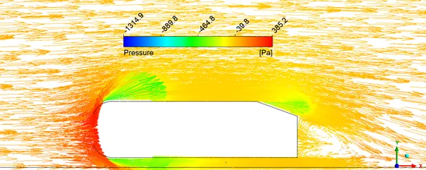
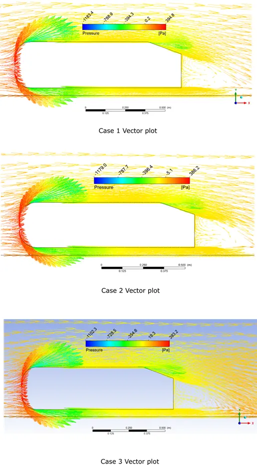
The plot represents the vector plot. The length of vectors resembles the magnitude and color variation has been done based on pressure.

Upon Running the base case, inference has been made that the area near the car body needs refining for better study.

For achieving the objective, the study has been divided into three cases as follows,

A second enclosure under the first enclosure has been made. The dimension of which has been discussed as follows.

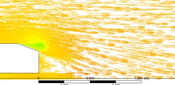
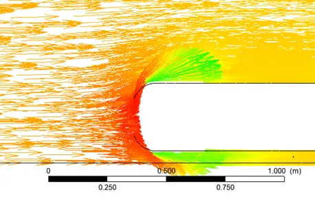
The Pressure Legend is same as that of above vector plot. The length of vector refers the magnitude of the velocity.

Trailing side of the model

Front side of the model

Front view for height and width of second enclosure.

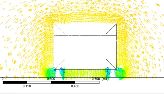
Upon measuring the distance around the body with big velocity vectors and high-pressure zones.

In the trailing end, the second enclosure has length of 1m, whereas it begins 0.3m before the car body. The height of second enclosure is set to 0.3m.

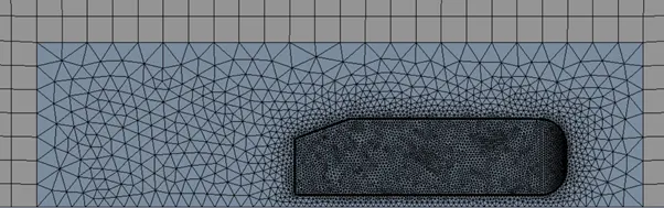
Mesh With Second Enclosure

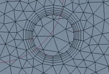
Meshing of the pillar.

Since the plane of symmetry as been introduced in the further models, so the reference area has been halved.

Later, the mesh size has been varied based on 3 parameters, namely – second enclosure, the surface of car model, inflation layer.

Case 1

The inflation layer has 5 layers of which, the first layer has height of 0.001m

The second enclosure has the element size of 0.05m

In the vicinity of face of car body, the element size is of 0.01 m

Near the pillars the element size is of 0.005m

The domain is split in half along the plane of symmetry.

The total No. of elements are 293,163.

Case 2

The inflation layer has 5 layers of which, the first layer has height of 0.001m

The second enclosure has the element size of 0.05m

In the vicinity of face of car body, the element size is reduced to 0.008 m

Near the pillars the element size is of 0.005m

The domain is split in half along the plane of symmetry.

The total No. of elements are 416,945.

Case 3

The inflation layer has 5 layers of which, the first layer has height of 0.001m

The second enclosure has the element size of 0.02385m

In the vicinity of face of car body, the element size is 0.01 m

Near the pillars the element size is of 0.008m

The domain is split in half along the plane of symmetry.

The total No. of elements are 498,936.

Results and Discussions

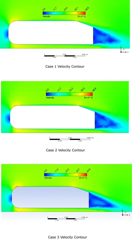
Velocity Contours

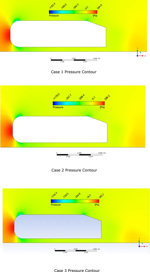
Pressure Contour

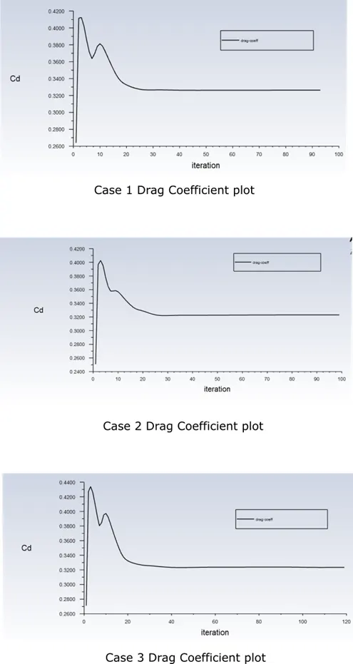
The drag coefficient plot

The vector plots

Separation of Flow

The point from where stream of fluid appears to get separated from the contour of the body in flow, is called the point of separation. From the vector plot, it can be observed that in the trailing end the zone comprises of negative pressure, and vectors appear to rollback in the direction opposite to that of the bulk flow. It marks the point of separation in the present case.

On Observing the simulated results, it is evident that whenever the cross-section of the flow changes, there is low pressure region behind the object and high-pressure region ahead of the object. The low-pressure region often comprises of velocity vectors in opposite of bulk from direction. The negative pressure appearing in the results are due to pressure less than atmospheric pressure. So, the pressure becomes negative.

Comparison of coefficient of drag and lift for the three cases.

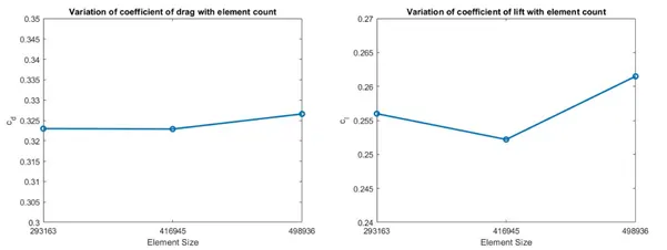
Upon running the simulation for differenrt grid size and changing mesh in different regions, it can be inferred that, the increase in mesh in the second confined enclosure gives approximate coefficient of drag to be around 0.33

Further the region can be more refined and the first layer thickness can be diminshed to better correlation with the experimental results.