Week 3 - External flow simulation over an Ahmed body.
Challenge: External flow over an Ahmed’s Body.
Q1. Describe Ahmed’s body and its importance.
Ans. The Ahmed body represents a simplified, ground vehicle geometry of a bluff body type. Its shape is simple enough to allow for accurate flow simulation but retains some important features relevant to automobile bodies. This model describes how to calculate the turbulent flow field around a simple car like geometry.
The air flow around the Ahmed body captures the essential flow features around an automobile. Its physical significance is very much practical, as the model is used to describe the turbulent flow field around a car like geometry. Ahmed body simulation is used to calculate the drag force which experience by a car body in real life scenario.
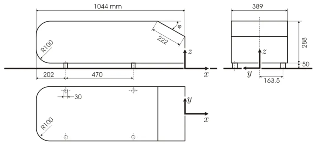
The Ahmed body was described originally by S. R. Ahmed in 1984 [1]. Three main features were seen in the wake:
1. The A recirculation region that is formed as the flow separates at the top of the vertical back surface of the model.
2. The B recirculation region that is formed due to the separation at the base of the model.
3. The c-pillar vortices that form as the vorticity in the side boundary layers roll up over the slant edges.
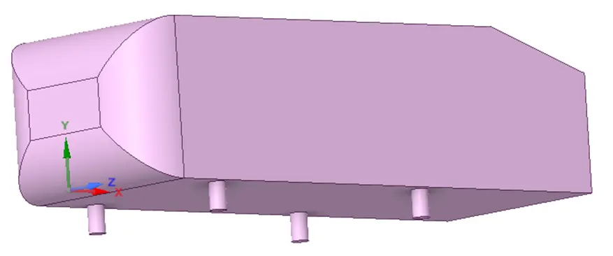
Fig.1 Ahmed Body in 3D
Purpose: By this simulation, we aim to get the velocity magnitude, pressure magnitude, wake region, drag force and lift force on the car body.
Grid Independency test:
Firstly, we have done the base line arrangement for doing CFD analysis.
Enclosure: To create the wind tunnel, it is very easy to create the wind tunnel with this option. For creating the box in the outer portion of the body. Select the enclosure option and click on the body. To edit the box, just un-tick the symmetry option & create the box around the body.
Dimension of the wind tunnel.
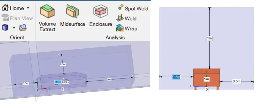
As CFD codes assumed, the variation of the velocity, temperature, pressure etc. across cells in the mesh is linear. So, we have created a box near to the Ahmeds body for local refinement of the mesh. So that we can measure the velocity analysis & other CFD data analysis efficiently.
After creating the double enclosure, it should be ensured that both of the boxes should share the data across the boundary. So that we have selected the share option for both the enclosures.
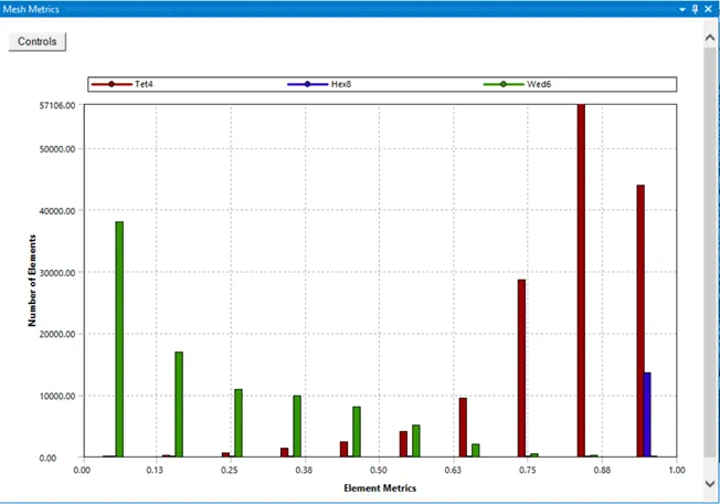
Meshing of the body: Outer body of the wind tunnel, we have used tetrahedral mesh, as this mesh can give proper results with least interference to the overall flow simulation. For creating tetrahedral mesh we have used ‘Multizone’. In the field of “methods’.
Size for the ‘Tetrahedral’ mesh is 100 mm. To create the even sized mesh, we have also defined the max size of the mesh size is 100 mm.
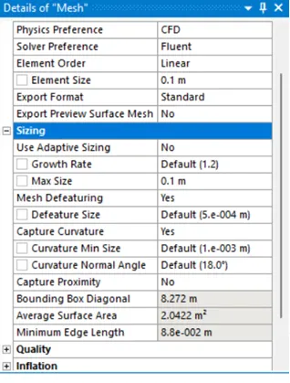
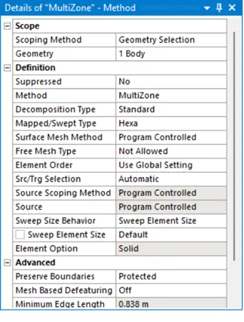
For creating local refinement much effective, we have make the mesh size much lower as compared to the outer body of the mesh. Mesh size for local refinement is 50 mm. For creating the local refinement much lower than the outer body, we have used the ‘Body Sizing’ and select the inner box of the wind tunnel.
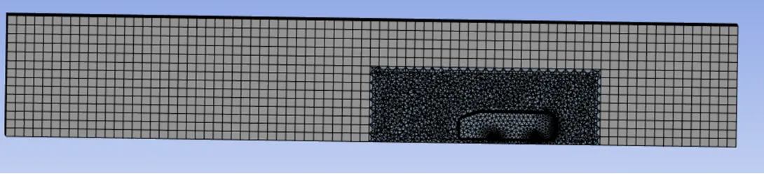
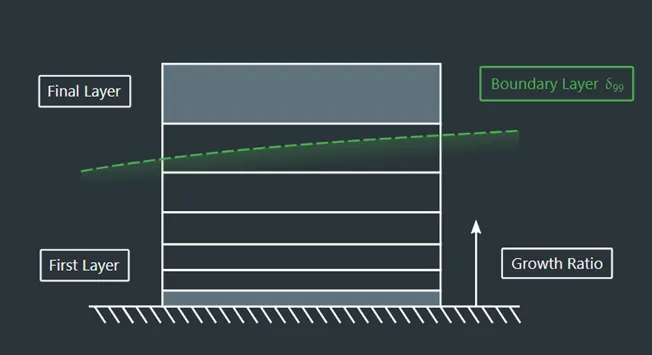
Inflation layers: Inflation is the process of creating a fine mesh or layers of fine mesh on the area of interest in the domain. Inflation layers used in CFD simulation to create the thin layer near the body in interest. We have to create the inflation layers up to the boundary layer or above the boundary layer.
Boundary layer: The boundary layer is a thin layer of a real fluid along the surface of an object in which viscosity affects fluid dynamics. When fluid flows over a plate, velocity near the surface in much lower and vorticity is present. The no-slip condition accounts for zero relative velocity at the plate and keeps on increasing until it reaches the free steam velocity. The thickness if the boundary layers along the lengths of the plate. In a narrow boundary layer adjacent to the plate, the shear forces and inertial forces are equally important in determining the motion of the fluid element and outside of the region, shear stress can be neglected. The thickness of the boundary layer is often describe as the distance from the plate until the velocity reaches 99% of the free stream velocity.
Describing first layer thickness of inflation layer: For describing the first layer height for the inflation layers, firstly we have to define the value of ‘Y+’ for getting the first layer thickness.
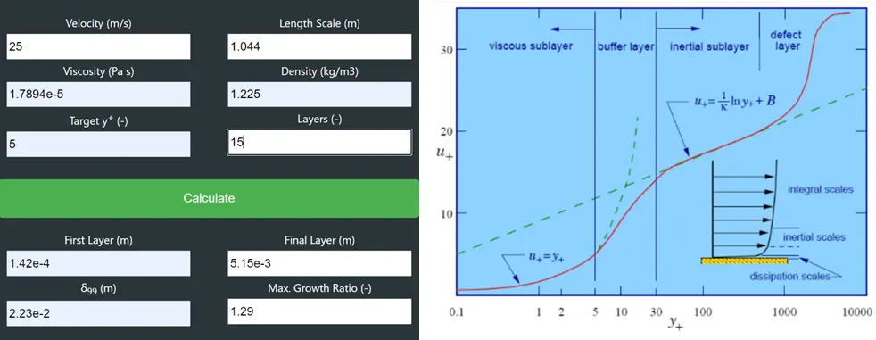
The laminar sub layer is also called the viscous sub layer, is the region of a mainly turbulent flow that is near to no slip boundary and in which viscous shear stresses are important. As such it is a type of boundary layer. The existence of the viscous sub layer can be understood in that the flow velocity decreases towards the no-slip boundary.
As we have to capture the all-possible changes & events near the wall boundary, so it is advised that the mesh count should be as large as possible to capture all the possible changes near the wall boundary. And it is also observed in the above diagram that the curved small dotted line is a linear variation between y+ & u+ in the laminar sub layer, but it follows the direct numerical simulation (red thick line) results only up to y+ of 5. So, it is decided to choose the y+ value to 5 only.
Calculator value –
Inlet Velocity – 25 m/s
Characteristic length – 1.044 meter
Density – 1.225 kg/m3
Viscosity - 1.7894e-5
Target y+ - 5
Layers – 15
By these parameters, the calculated values are;
First layer height is 0.000142 mm.
Growth ratio - 1.29
δ99 (m) – 2.23e-2
as we know that the boundary layer thickness δ99 to be contained within the total height of the inflation layer.
So, we can get the total height of the inflation layer from these formulae.
Yt = Yh x 1-G^n/1-G.
By this calculation, we got the total height of the inflation layer is 0.0218 mm and the boundary layer height is 0.023mm. So we have to change the total numbers of the inflation layers, so that the inflation layer can contain the boundary layer fully.
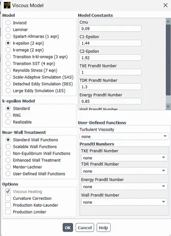
Viscous model: For this simulation, we have selected ‘K-epsilon’ model as it works well for a wide range of applications, suitable for both internal & external flows and it resolves the boundary layers effectively.
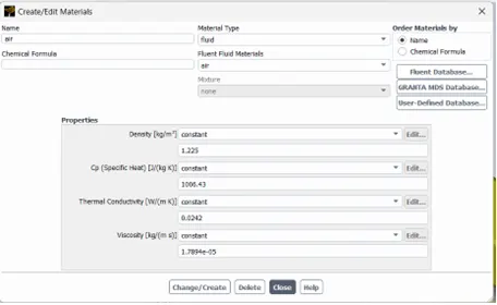
Material Selection: Air is taken as the material with default properties.
For this simulation, we have used density-based solver, because when the mac number is .3 and above, it is suggested to use density-based solver, because we have to take the compressibility effects.
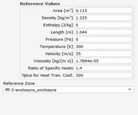
Reference Values:
Inlet Velocity is 25 m/s.
Case -1
With refined mesh & numbers of element is 251365. Inner shell size – 50 mm
By this simulation, total drag coefficient is 0.38, and it is coming with in the standard value for the drag coefficient for the car.
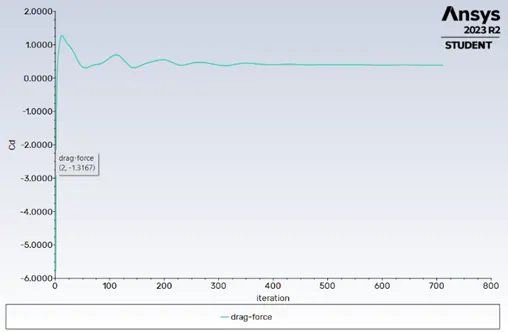
Drag Coefficient Plot
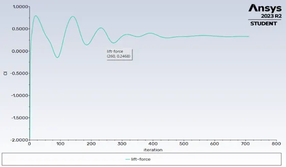
Lift Coefficient Plot
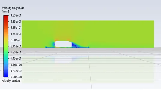
Velocity Contour
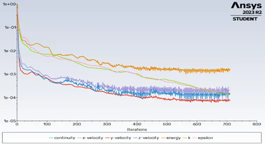
Residuals

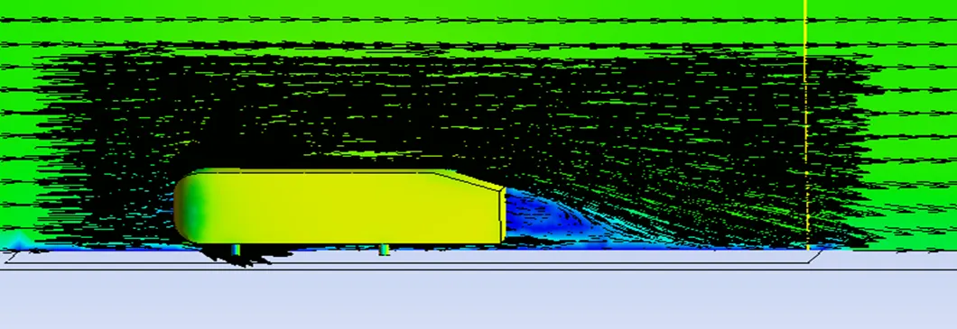
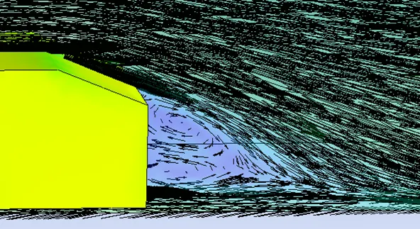
Vector Plot of velocity
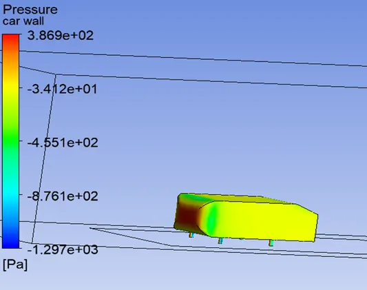
Pressure on Ahmeds body
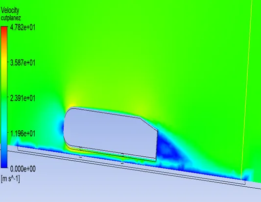
Velocity Distribution on Plane
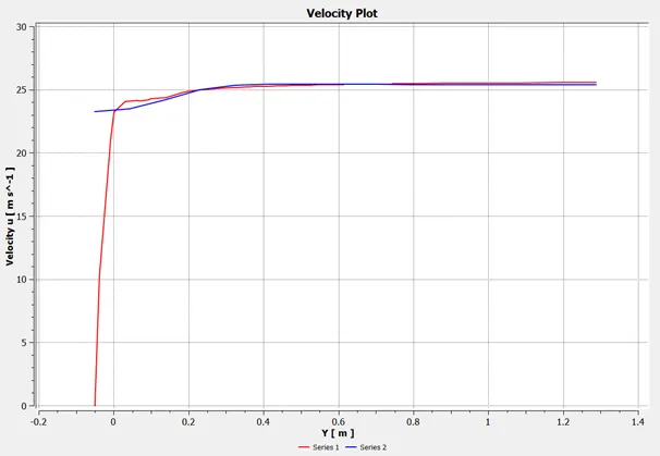
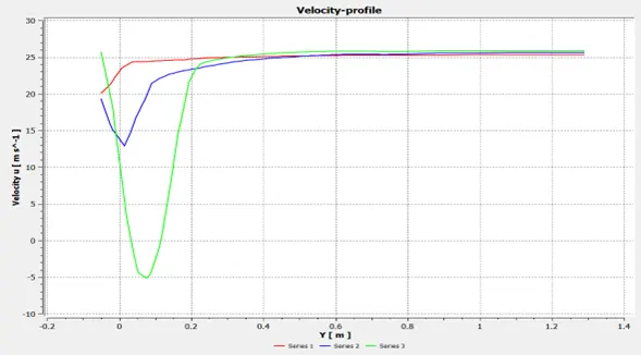
Velocity plot of different location at the cut plane.
Case 2 :
Number of element – 427338.
Inner domain element size – 40 mm.
Inflation layer- First layer height – 0.000142 mm.
Number of inflation layer – 16
Growth ratio – 1.25
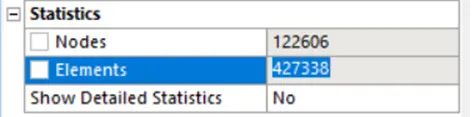
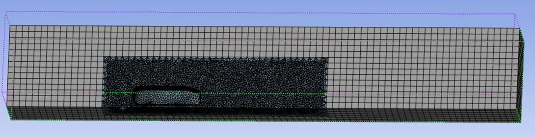
Final Mesh body, with 40 mm inner domain shell size.
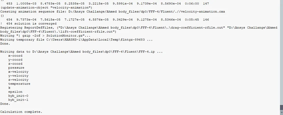
Solution is converged at the 454 iterations.
By this solution, we got the minimum drag force at 159 iteration is 0.3062, but the drag coefficient at the 454 iteration is 0.42. By this we got to know that, increasing the mesh element does not give the results with major difference.
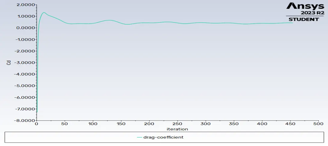
Conclusion on the final result:
Grid dependency test allow us to analyse the different result with different mesh size. As we make the mesh size finer, the velocity vector plots are becoming much finer & smoother with increasing number of the total mesh shell count.
Clearer picture of the wake region can be seen, when the mesh is becoming clearer.
As the CFD results are linear to the mesh centroid. So, we can say that, when the mesh is becoming more finer, we got the finer result & smooth velocity transition.
Conclusion over negative pressure on the Ahmeds Body.
After concluding three mesh & final results. We can see that there are some areas where pressure is negative. There are many reasons by which, the pressure on the car wall body become negative.
When the air moving over the vehicle is separated at the rear end. It leaves a large low pressure turbulent region behind the vehicle known as the formation of pressure drag, which is eventually reduces the vehicle performance.
The region of recirculating flow immediately behind a moving or stationary blunt body, caused by viscosity, which may be accompanied by the flow separation and turbulence flow, or the wave pattern on the water surface downstream of an object in a flow, or produced by a moving object caused by the density differences of the fluid above and below the free surface and gravity.
When the vehicle is moving at a certain velocity, the viscous effects in the fluid are restricted to a thin layer called boundary layer. Outside the boundary layer is the inviscid flow. This fluid flow-imposed pressure force on the boundary layer. When the air reaches the rear part of the vehicle, the fluid gets detached. With in the boundary layer, the movement of the fluid is totally governed by the viscous effect on the fluid. The Reynolds number is dependent on the characteristic length of the vehicle, the kinematics viscosity and the speed of the vehicle. The fluid moving around the vehicle is dependent on the shape of the vehicle and Reynolds number. There is another important phenomenon which affects the flow of the car and the performance of the vehicle. This phenomenon is commonly known as the wake of the vehicle. When the air moving over the vehicle is separated at the rear end, I leaves a large low pressure turbulent region behind the vehicle known as the wake. This wake contributes to the formation of the pressure drag, which is eventually reduces the vehicle performance.