Week 3 - External flow simulation over an Ahmed body.
Q1. Describe Ahmed's body and its importance.
Aim
To perform external aerodynamic simulation over an Ahmed body and calculate drag and lift coefficient for a free stream velocity of 25 m/s. Also perform mesh independence test
Introduction
The Ahmed body was at first put forward by Ahmed et al. (1984). is a general car model which is used by the automotive industries (Morel (1978), Good and Garry (2004), Guilmineau and Chometon (2009), Heft et al. (2012) and Huminic and Huminic (2012)), to examine the wake forces and dynamics which is experienced in a variety of configurations. The Ahmed body is designed to have a smooth-edged front end with a flat roof and a flat bottom section and an angled back slant which basically acts as the rear window of a car and ending with a vertical base. The back-slant angle which is commonly designated as ϕ is very critical to the flow patterns which are fashioned at the near wake region and subsequently has an impact on the aerodynamic forces which act on the body.
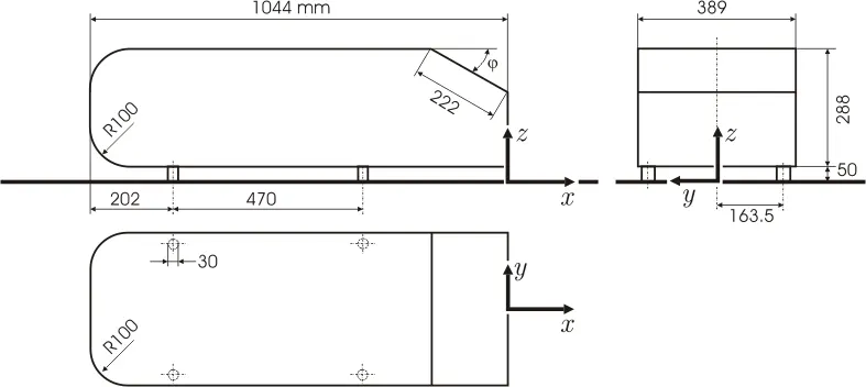
Theory[1]
The Ahmed body was described originally by S. R. Ahmed in 1984. Three main features were seen in the wake:
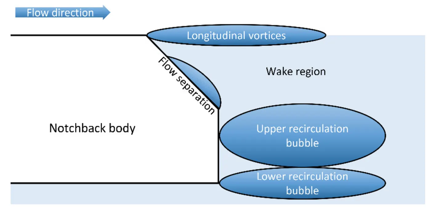
1. The A recirculation region that is formed as the flow separates at the top of the vertical back surface of the model
2. The B recirculation region that is formed due to the separation at the base of the model.
3. The c-pillar vortices that form as the vorticity in the side boundary layers roll up over the slant edges.
The wake was shown to be highly dependent on slant angle. For slant angles less than 12°, the flow remains attached over the the slant. The flow is essentially two-dimensional and has low drag. Between 12° and 30° the flow becomes much more three-dimensional as the c-pillar vortices form. These reach maximum strength at 30°. The drag increases significantly as the low pressure cores act on the rear surfaces. Past 30° the flow separates fully off the slant. This results in a sudden decrease in drag and weaker c-pillar vortices.
importance in practical applications [2]
The Ahmed body is a generic car body (a simplified vehicle model). The airflow around the Ahmed body captures the essential flow features around an automobile and was first defined and characterized in the experimental work of Ahmed. Although it has a very simple shape, Ahmed body allows us to capture characteristic features that are relevant to bodies in the automobile industry. This model is also used to describe the turbulent flow field around a car-like geometry. Once the numerical model in validated, it is used to design new models of the car. Car companies makes numerous attempts to develop modified designs to effectively reduce the aerodynamic drag force which occurs at the rear end without putting any constraints in the stability, comfort and safety of the passengers.
Pre-processing and solver setting - Solving & Modelling approach
Spaceclaim Operations
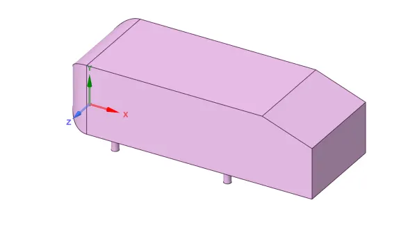
Ahmed body is imported in spaceclaim using import geometry option available with the geometry tab in the workbench.
Right-click on geometry > select open with space claim. Now drag the solid part to the space claim window and it gets uploaded.
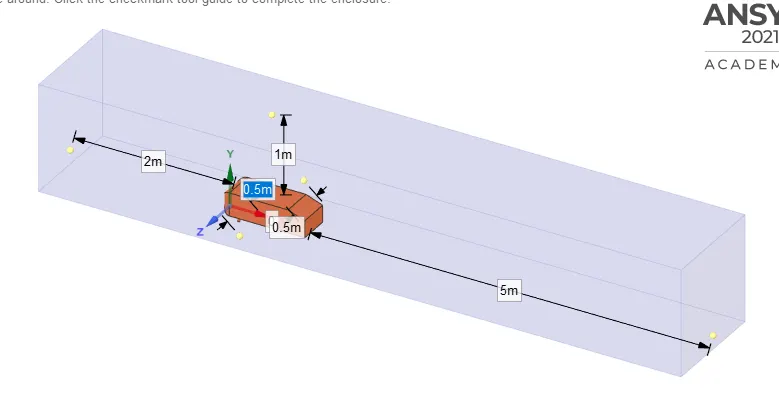
go to prepare > select enclosure > select the Ahmed body > give the appropriate dimensions > and click the tick mark. This will create a wind tunnel structure.
Envelope is created around the body concidered as a control volume of flow over ahmed body. The dimention of control volume is given below-
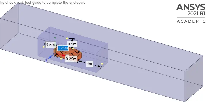
To capture the physics more accurately around the Ahmed body we create a small envelope around a body as a refinement zone. The dimension of refinement zone is given below-
As the body is perfectly symmetric, we can run the simulation by considering the only half body. This is the best practice where you can save on the number of cells and get the results faster as well. The Ahmed body geometry is modified using 'split body' command in SpaceClaim to cut the body exactly symmetric and using its half symmetric part we can procceed for other manipulations.
After using split command on the above body the operated body is shown below-
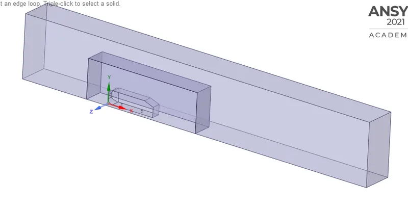
Check for inteference and fix the interfering part and go to section view to check for non-inteference which is shown below-
Go to prepare > select the interference and click the tick mark to remove the interference.
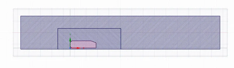
Meshing
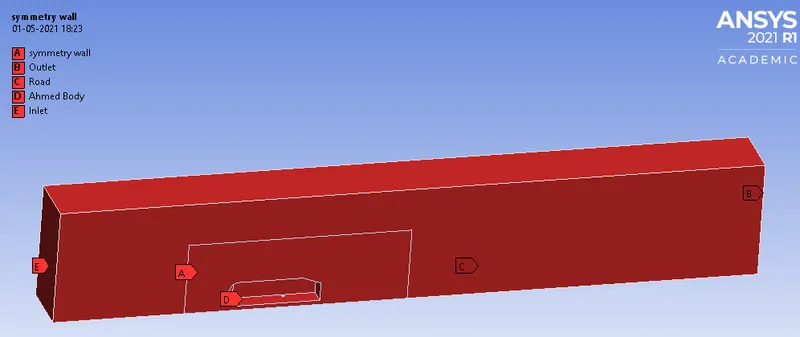
Here we start with creating named selection. Select face selection > then select a face and click N and name the selections. Four named selections must be created, namely, inlet, outlet, car wall, and symmetry wall (wind tunnel wall)
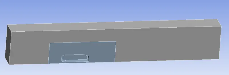
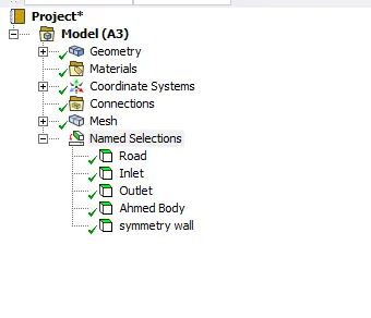
Mesh Operations and Refinements
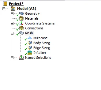
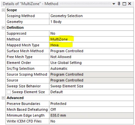
As we have two envelope and we are trying to create two different type of meshing for this problem therefore we use multizone mesh. The MultiZone mesh method provides automatic decomposition of geometry into mapped (structured/sweepable) regions and free (unstructured) regions. It automatically generates a pure hexahedral mesh where possible and then fills the more difficult to capture regions with unstructured mesh. [3]
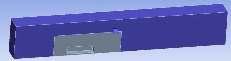
After going for base line meshing we undestand which are the area of concentration to see the better physics around the ahmed body and within the computational domain. Thus we go for certain mesh refinement techniques to refine the small regions and flow region.
to refine mesh of inner envelope we go for body sizing
Rt click mesh -> insert -> Sizing- selet the inner domain as a body and give the element size
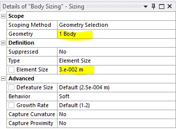
To refine the area around thw wheels of ahmed body go for edge sizing
Rt click mesh -> insert -> Sizing- selet the edges of wheels and give the no. of division
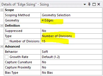
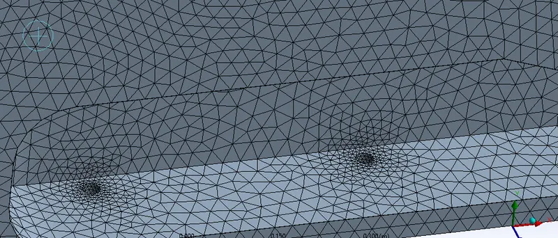
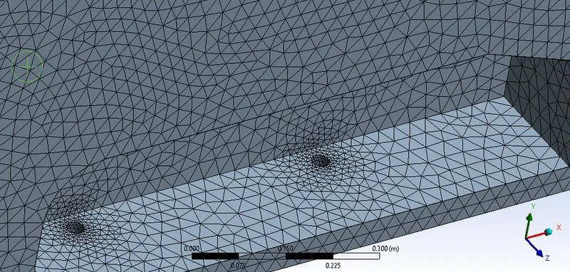
To define the boundary layer effect on ahmed body we go for adding inflation layers to ahmed body
Rt mesh -> Insert -> Inflation - here we use inflation option as first layer thickness to calculate the first layer thickness we use y+ calculator
https://www.pointwise.com/yplus/index.html
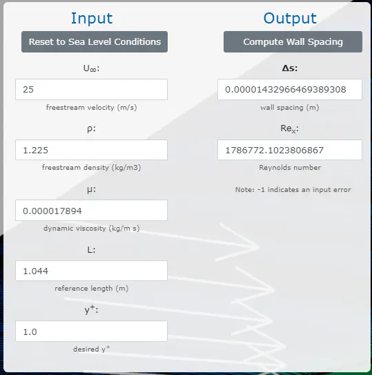
here the free stream velocity is given in problem statement i.e. 25m/s and the as air is our working fluid thus air properties are given(density and viscocity). The reference length is Ahmed body's length and for k-w SST turbulence model y+ value is concidered in between 1 to 5 this we take 1 for better results.
Thus the obtained `Delta`S value is required first layer height we put in inflation details and we give 10 no. of inflation layers with a growth rate of 1.2
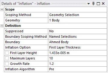
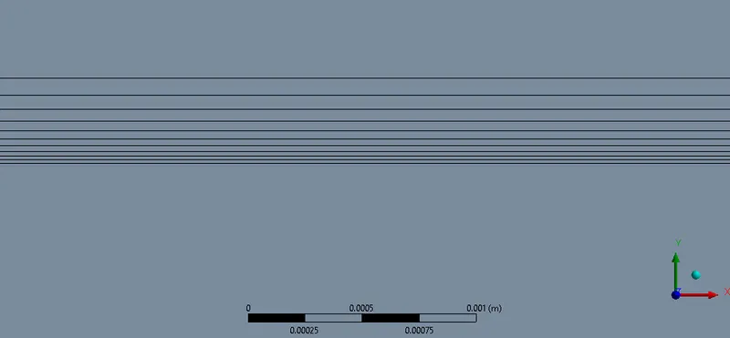
Performing all the mesh operation and refinments we obtained our required mesh for simulation
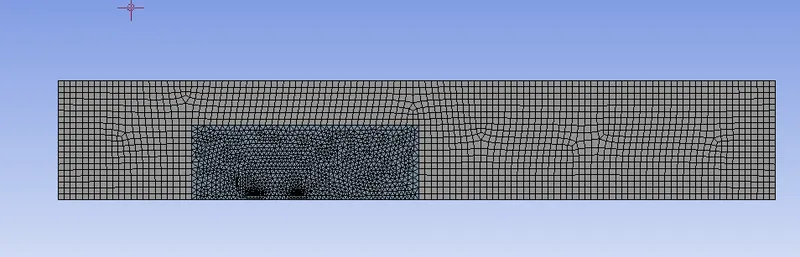
To obtain better results the quality of mesh is required and to obtain mesh independent results we need to perform grid independency test.
Solver Setting
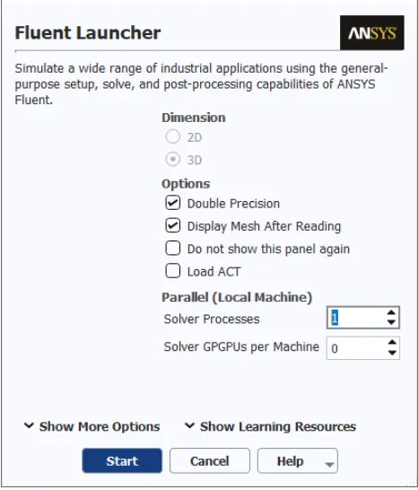
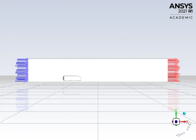
Model Selection: -
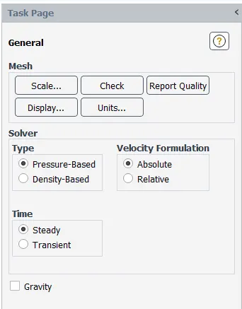
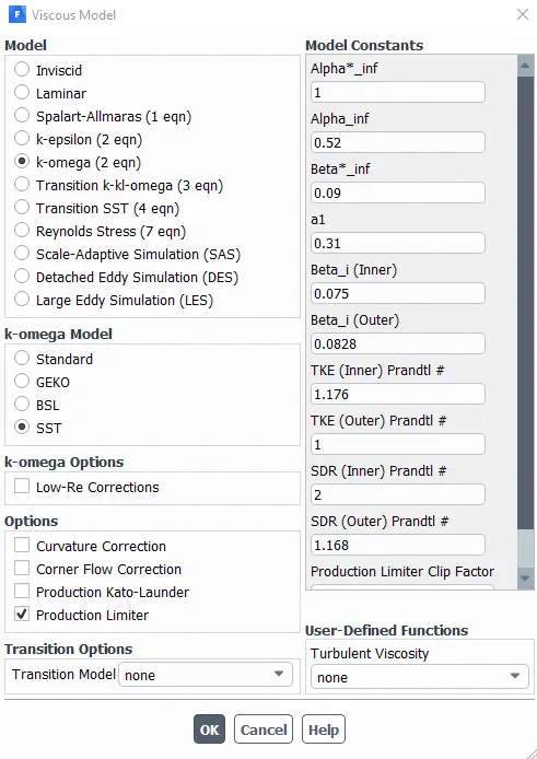
Steady state flow witrh the pressure based model is selected for the simulation. K-w SST turbulence model is taken as it has low y+ value, gives the result accuracy as the flow is captured at the boundary layer viscous sub layer region.
Material Properties:
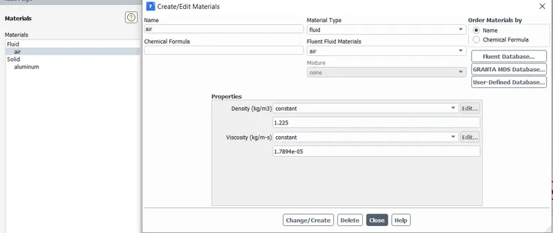
Boundary conditions:
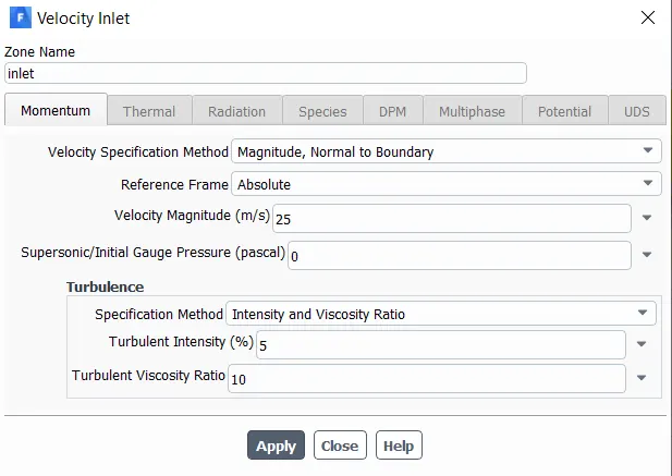
Pressure outlet: 1 atm
Ahmed body: No-slip
Symmetry: Walls of the enclosure
Methods:
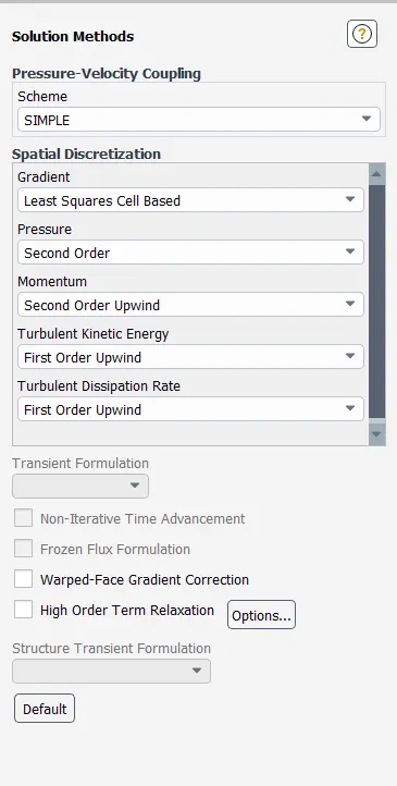
Initialization: Hybrid
Iterations: 500 to 600 iteratrion.
CASE 1 - Refined Case with a outer region element size of 0.07m & inner region element size of 0.045

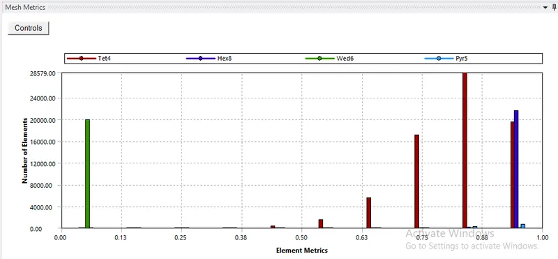
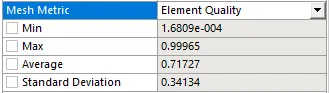
Element Quality
Aspect Rato
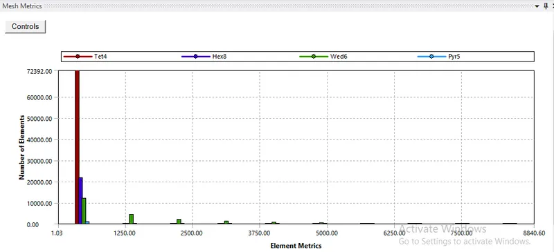
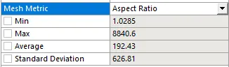
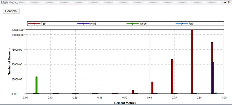
The generated mesh is refined from of baseline mesh with the element size of 0.07m of external and 0.05m internal enclosure. The mesh has generated 114697 total no of elements which is within the computational capabalities also the element quality is below 1 and the aspect ratio is above 1.3 as required. In grid independency test we taste for different element size of mesh and keeps on refining it till we get the steady i.e. mesh independent results.
Residuals
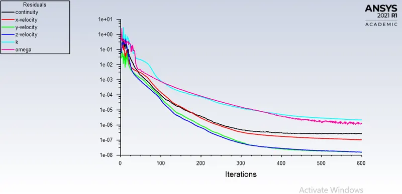
All the residuals falls below the 1e-3 that means the case has converged.
Drag Cofficient
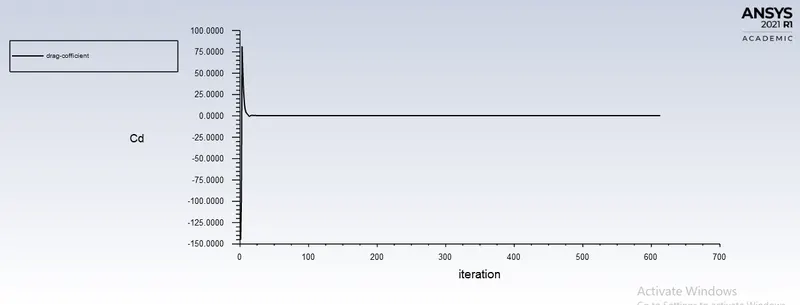
for the 1st refinement case the drag cofficient is found to be 0.28735602
Lift Cofficient
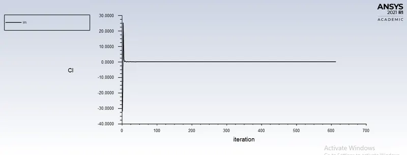
the lift cofficient is 0.15666182
Velocity Contours
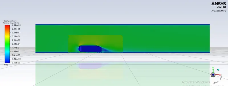
Velocity contours shows the velocity distribution around the body and within the computional domain.
Pressure Contours
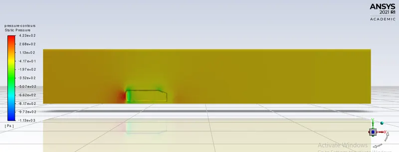
Pressure contours shows the pressure distribution over a ahmed body and within the computional domain.
Vector Plot - showing the wake region
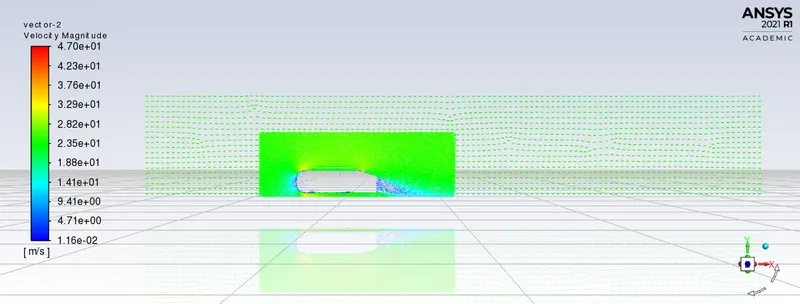
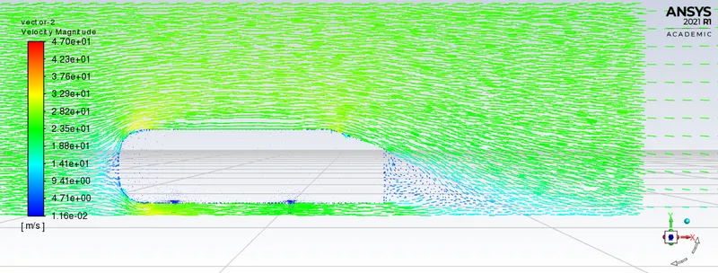
Vector plot shows the flow direction of velocity vectors.
All of the required physics i.e wake region is captured in this case but still we cant be sure with obtained drag and lift cofficient values thus to see the effect of refinement on obtained results we go fpr second refinement.
CASE 2 - Refinement 2 with a outer region element size of 0.06m & inner region element size of 0.04
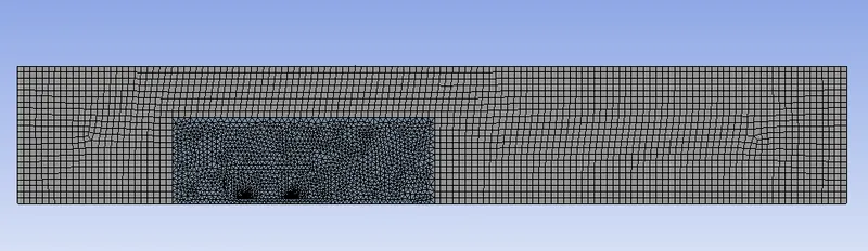

Element Quality
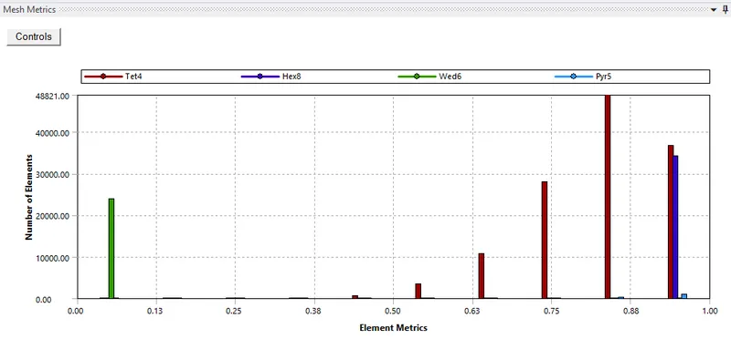
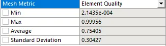
Aspect Ratio
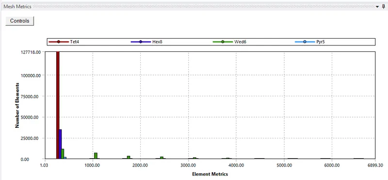
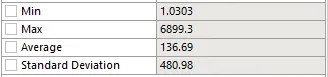
The generated mesh is refined from of case no. 1 with the element size of 0.06m of external and 0.04m internal enclosure. The mesh has generated 186756 total no of elements which is within the computational capabalities also the element quality is below 1 and the aspect ratio is above 1.3 as required.
Residuals
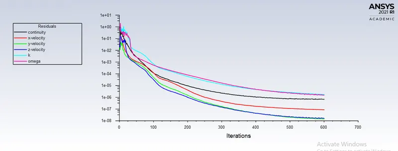
All the residuals falls below the 1e-3 that means the case has converged.
Drag Cofficient
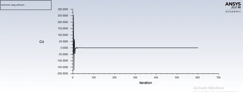
drag coff obtained is varried from 0.28(from 1st case) to 0.27866086. Thus the results of drag coff. varried from previous case.
Lift Cofficient
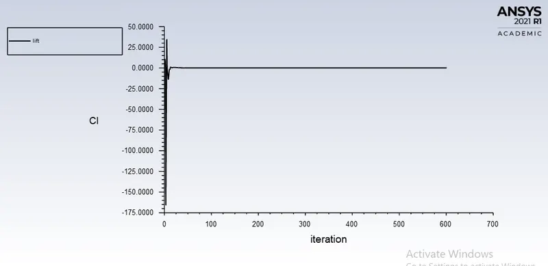
Lift Coff is also slightly varried from previous case 0.15907829
Velocity Contours
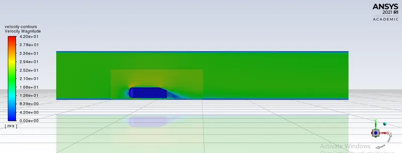
Velocity contours shows the velocity distribution around the body and within the computional domain.
Pressure Contours
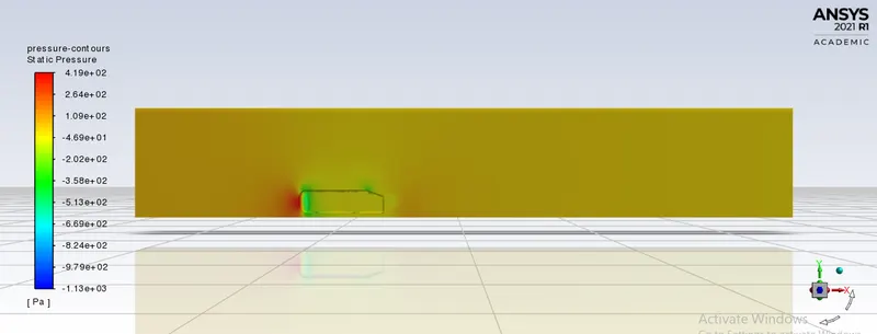
Pressure contours shows the pressure distribution over a ahmed body and within the computional domain.
Vector Plot - showing the wake region
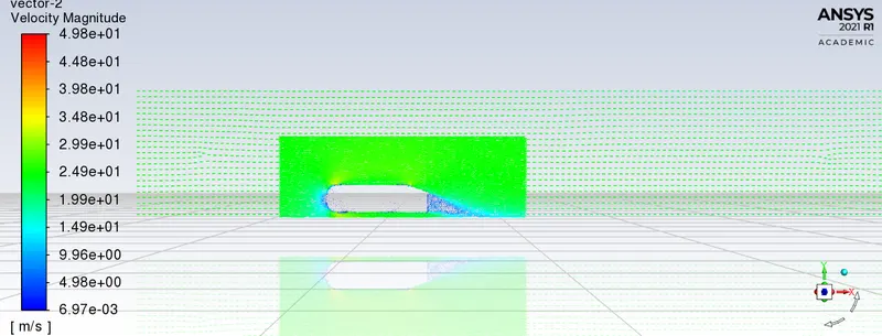
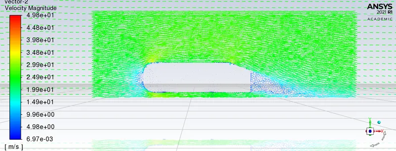
Vector plot shows the flow direction of velocity vectors.
Thus the results of drag cofficient and lift cofficient is varried from 1st case to second case. Lets see the the effect on results on further refinement.
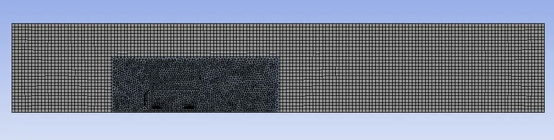
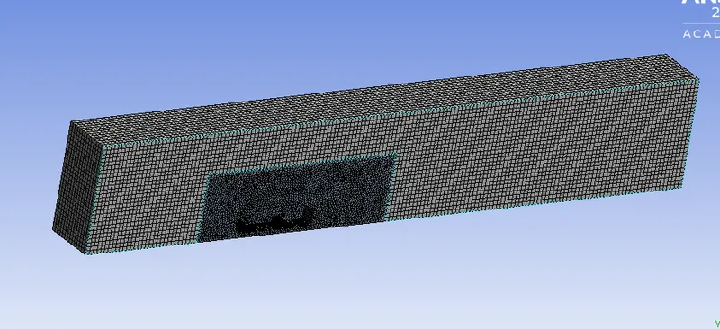
CASE 3 - Refinement 3 (final case) with a outer region element size of 0.05m & inner region element size of 0.03

Element Quality
Aspect Ratio
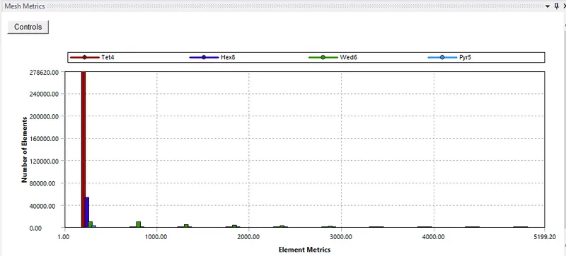
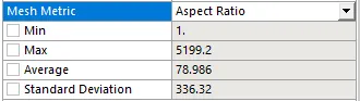
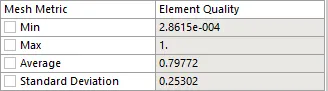
The generated mesh is refined from of case no. 2 with the element size of 0.05m of external and 0.03m internal enclosure. The mesh has generated 361617 total no of elements which is within the computational capabalities also the element quality is below 1 and the aspect ratio is above 1.3 as required.
Residuals
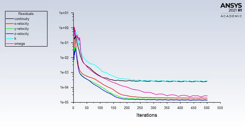
All the residuals falls below the 1e-3 and obtained a steady state in 250 iterations(which is less as compare to other two cases) that means the case has converged.
Drag Cofficient
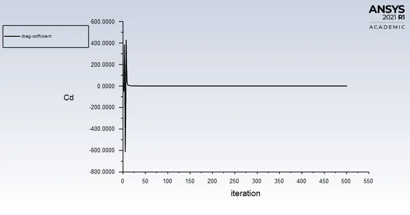
the drag coff reduces to - 0.25126234
The analatical drag cofficient is 0.33(mention in problem statement)
% error = ((0.33-0.25)/0.33)*100 = 24%
Thus we can say that our simulation is perfectely solved.
Lift Cofficient
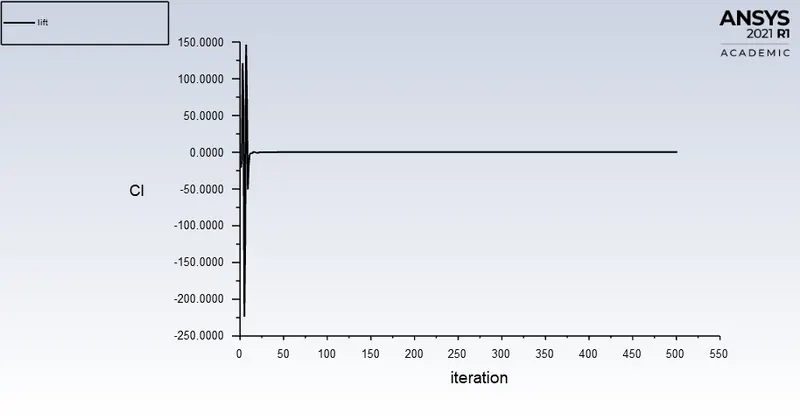
Lift coff is obtained to be - 0.16121879
Velocity Contours
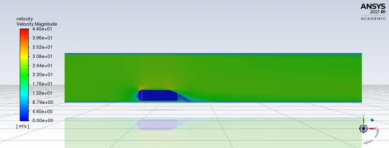
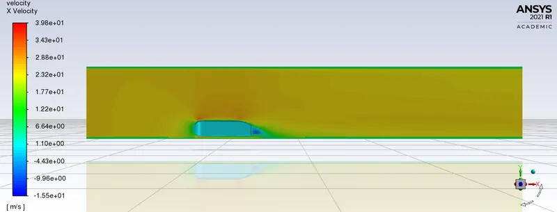
If we compare this case velocity contours with other two case then we can see that the wake region shown in this case has a more definite shape than other two cases and this is due to highly refined mesh.
Pressure Contours
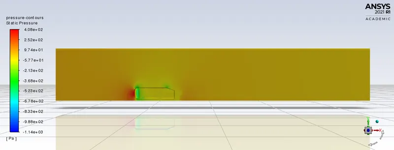
The frontal region of Ahmed body is flow impacting region which generates high static pressure. In this case the impacted region and negative pressure region can be seen accurately.
Vector Plot - showing the wake region
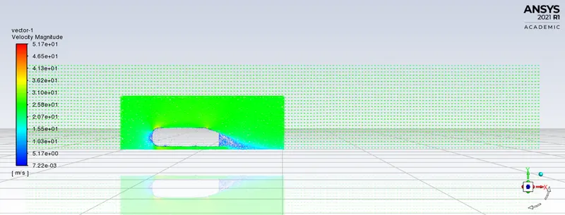
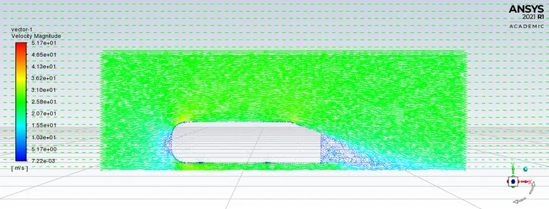
The vector plot clearly shows that the recirculated region is formed behind the ahmed body which has low velocity and the air is forming eddies behind the ahmed body.
Conclusion/ Inferences
1. Grid Independence Results
| Cases | Element Size | Drag Cofficient | Lift Cofficient |
| Case 1 | 114697 | 0.287 | 0.156 |
| Case 2 | 186756 | 0.27 | 0.151 |
| Case 3 | 361317 | 0.25 | 0.16 |
The above table is showing the all 3 different case data of drag and lift cofficient and these 3 cases are taken for finding grid independence taste. After reducing the element size below 0.05 and 0.03(case 3) the results obtained were the similar with case no 3 thus the optimum mesh size for simulating flow over ahmed body is case no 3.
The grid dependency test allows us to see smoother velocity profile. As we make the mesh finer i.e. when we increase the cell counts (closer to the limit), we can see from the vector plots from all the 3 cases, of the velocity that it becomes more and more smoother. One thing is observable that making the mesh finer lets us see the wake region more prominent. From the 3 cases, we can conclude that the flow is more defined at lower element size i.e. at case 3. The finer the mesh gets, the easier it gets in visualizing the contours. Mesh refinement increases the closeness of the resulting values to the true values.
2. Contours data
The graphical plots and contours for all three types of mesh are almost the same. Small differences are noticed in the appearance of the plots and contours but that is due to the difference in element quality. If we notice the velocity contour then we can see that the velocity around the wake region is high and low at the tail of the Ahmed body. If we connect this observation with the velocity vector plot then we notice that at the wake region the velocity vectors are large which is obvious due to the obstruction offered by the Ahmed body and at the tail of the body there is a circulating flow which is the reason for its low velocity. Whereas, for the pressure contours at the car wall and XY plane, high pressures are observed in the front of the body, and in the wake region we observe negative pressure.
Q2. Explain the reason for the negative pressure in the wake region.
Here We observed that a wake region(a large recirculation region) have established at the rear side of Ahmed body in velocity flow Which have created a vortex flow at rear side.
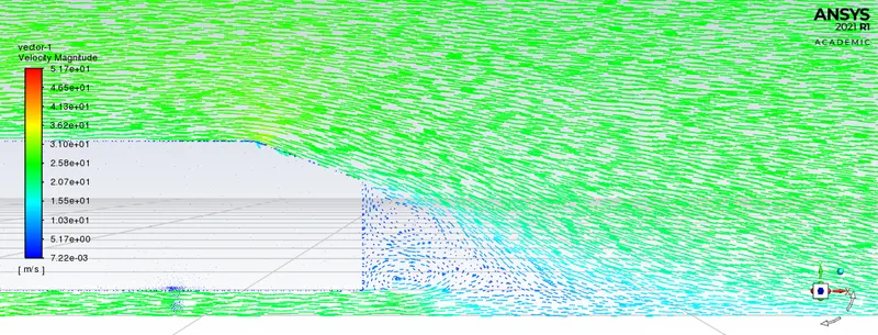
When the air moving over the vehicle is separated at the rear end, it leaves a large low pressure turbulent region behind the vehicle known as the wake. This wake contributes to the formation of pressure drag, which is eventually reduces the vehicle performance.
Formation of recirculation zone is also one of the reson for formation of negative pressure in a wake region.
Q3. Explain the significance of the point of separation.
When an object moves in a fluid the fluid sticks on the surface of the body and creates a boundary layer over it. Now for certain bodies and type of motion, there is a point on the body where the fluid detaches from its surface, thus breaking the boundary layer, this point at which the fluid detaches from the surface is called the point of separation. This flow separation takes place due to excessive momentum loss near the wall in a boundary layer trying to move downstream against increasing pressure, i.e., , which is called adverse pressure gradient which can be observed at the tail of the Ahmed body.
References
1. https://www.cfd-online.com/Wiki/Ahmed_body