Week 3 - External flow simulation over an Ahmed body.

Aim- External flow simulation over the Ahmed body.

Introduction – Ahmed body is a generic car model or a simplified car model, and the flow of air around the ahmed body capture the essential flow feature around an automobile, it is generally used in the CFD purpose, first invented by S.R. Ahmed in 1984.

Here in the week 3 challenge we are going to perform the fluent analysis over the body and going to measure the drag and lift coefficient over also the wake region which is causing the negative pressure region and the vortex formation behind the car model.

Procedure- the ahmed body have its standard dimension which is 1.044m in length, height is 0.288m and width is 0.389m. the solving and modelling approach is going to be covered in the following steps.

Step_1- setting up geometry in the space clan.

• Here the simulation is external thus we need to extract the model and need to create the wind tunnel type of enclosure around the body.
• Change unit to meter.
• The enclosure dimensions are 2m in front, 5m in back, 0in bottom, 1m for the top and 0.5-0.5m in both the sides.
• And create one more enclosure around the body so we can provide the separate target mesh length for both the case also we will have the gradually increasing mesh size.
• The second enclosure will have the 0.5m in front, 2m in back, 0m in the bottom, 0.5m in the top and 0.25-0.25m for both the sides.
• Use interference common to make it separate.
• Use split command to delete the half symmetry part, so we will have the half mesh elements to cover.
• Share topo will help in the flow of math equation in both the enclosure.

Step_2 mesh and the mesh independent study.

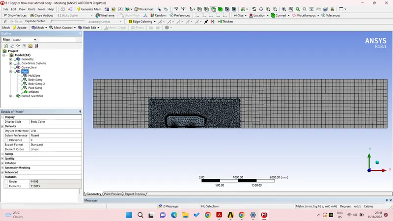
• Mesh independent study is the method of investigating whether the simulation result is being change with the number of mesh elements or not, thus for this we are going to create the three case with increasing element size and going to see the change in the drag and lift.
• Provide the name the curved front side is inlet the rear back side is the outlet, the side walls re symmetry walls, and the last car model.

Case	Base body	Car body	Face	No of element
Case-1	100mm	50mm	8mm	1,15,015
Case-2	80mm	30mm	6mm	3,29,949
Case-3	80mm	20mm	5mm	8,85,161

• Inflation layer the Y+ layer or prism layer is provided to compensate the phenomena of the boundary layer thickness here by the help of Y+ calculator by providing all the details we will have the three following important requirement to create the boundary layer.
• The first layer thickness is 0.5mm.
• The no of layers is 20.
• And the growth rate factor is1.2

Step_3 setting up the geometry or pre processing

• Quality check> type> pressure based solver as the flow is not compressible.
• Viscous model is k-epsilon SST.
• The method for solving is coupled.
• Steady state, the material is air.
• Under the boundary condition the inlet will have the velocity of 25m/s.
• The outlet will have the 0-gauge pressure.
• The wall is symmetry condition.
• Under the reference value we will have the front projected area and the values of material with the model length need to be updated.
• Under definition we will have the graph plot of drag and lift.
• Now initialize the solution.
• With around 100 iteration start the calculation.

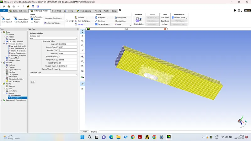
Result- Here we have to use the different mesh size start with large to small target length one after another to finalize the result and thus we need to refine the mesh quality for this we are going to do some improvement here.

• For this we are going to create the duplicate of the whole fluent model.
• We are going to do the local refinement, here we are running the base line setup generally need to do the iteration based on problem to problem.

Case	No of element	No of iteration	Drag coefficient	Lift coefficient	continuity
Case-1	1,15,015	100	0.3814	0.3116	1.9045*10^-04
Case-2	3,29,949	100	0.3349	0.2963	1.4757*10^-03
Case-3	8,85,161	200	0.3142	0.2793	1.0119*10^-03

The velocity, pressure, drag lift coefficient and the residual plots case by case are attached in the in the snapshot format.

Case_1

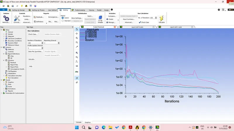
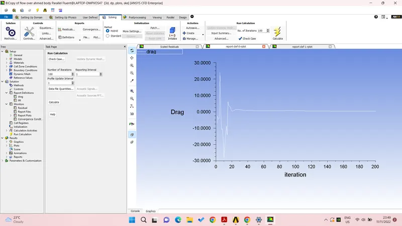
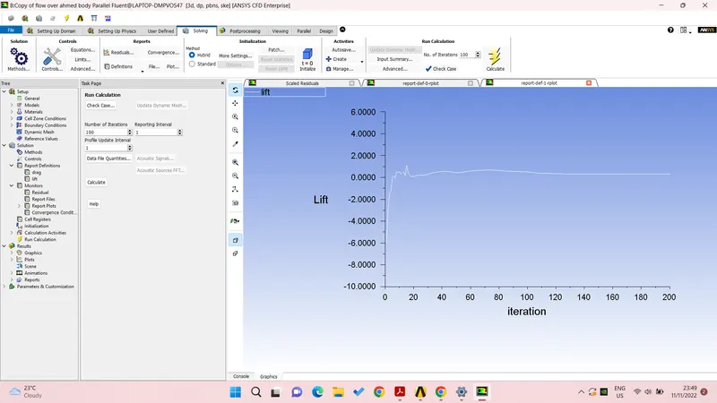
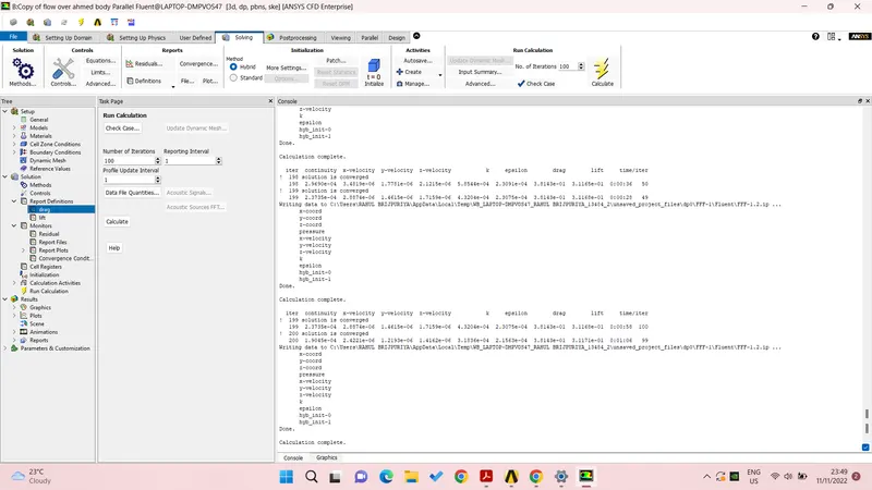
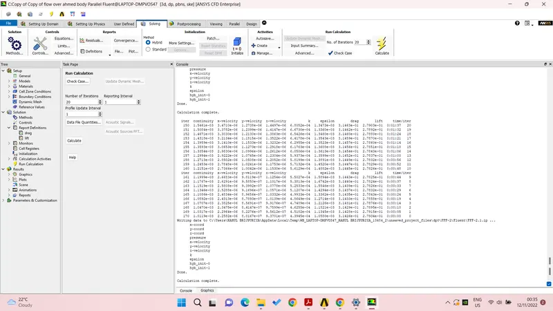
this console tab will show the end result after iteration, sime values like drag, lift and residual velocity, epsilon and continity we can see at the end solution is almost converged.

Case_2

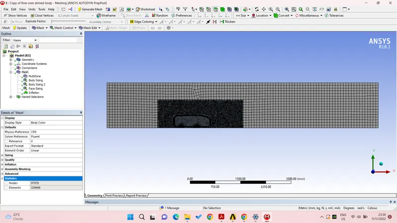
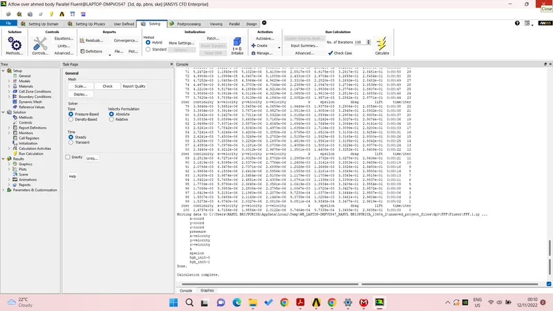
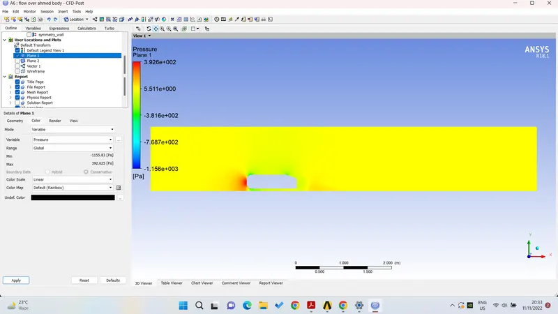
This image below shows the pressure contour here we can see the front notch has the high gauge pressure as the velocity head is converting into the pressure head. Also the back side has the vacuumed pressure which can be seen in the contour.

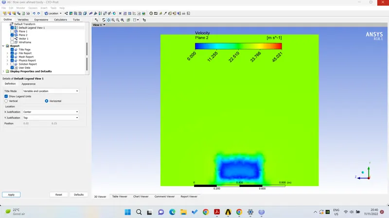
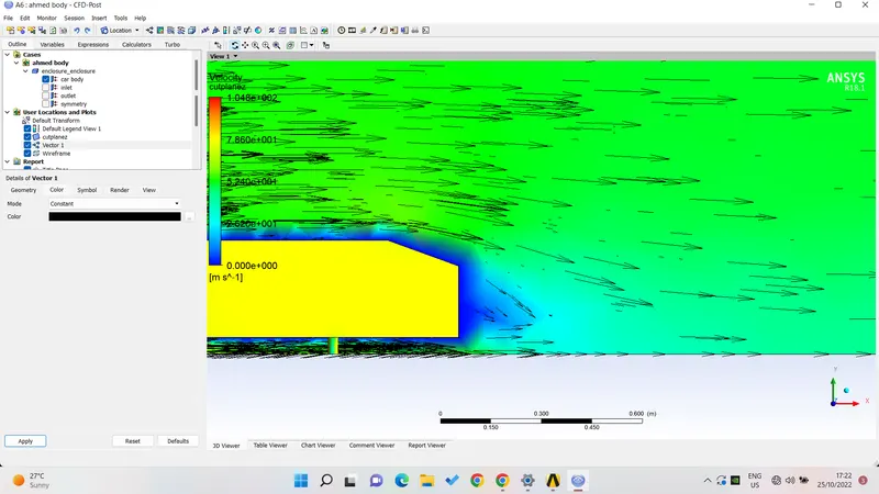
This is the plane in YZ axis showing the back side of the car model we can see at the center we have the zero velocity at the wake region.

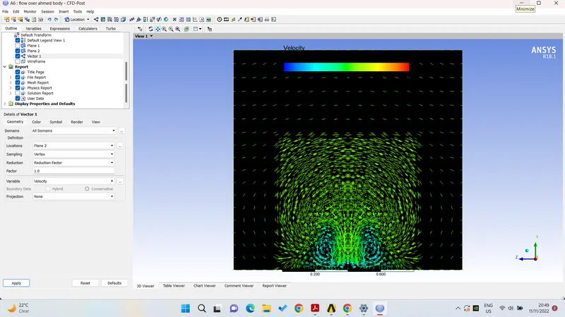
This is the vortex plot at the wake region, here we can see the vortex formation downstream to the model.

Case_3

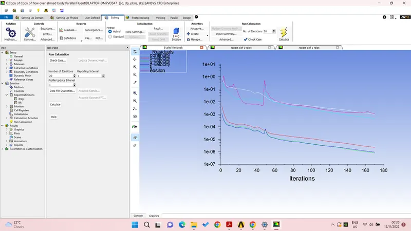
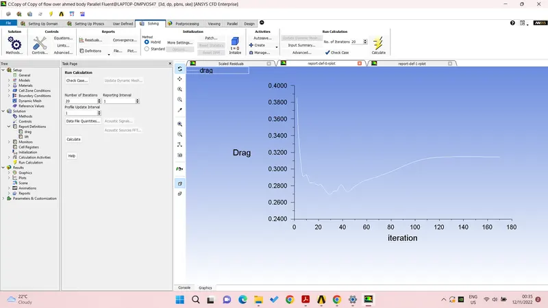
Here this image shows as the number of mesh element is increasing the more refine result of drag can be seen here, at first the drag value is going down but as the number of iteration increase the value is being converged.

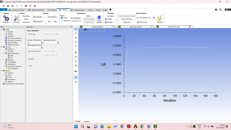
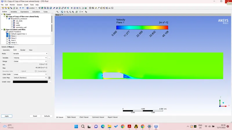
Here the result is more refined, as the number of mesh element is high so the mesh result is looking more on fine side.

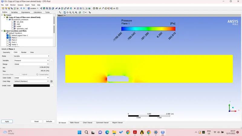
Also the pressure variation can be seen more on refined side varying on the

Learning outcomes- when a fluid is forced to flow over a curved surface at high velocities. A fluid follows the front portion of the curved surface with no problem, but it has difficulties remaining attached to the surface on the back side. At sufficiently high velocity, the fluid stream detaches itself from the surface of the body. This phenomenon called the flow separation.

The location of the flow separation depends upon the several factors such as the Reynolds number, the surface roughness, and the level of fluctuation in the freestream. The majorly it occurs at the Sharpe edges over the model.

And at the flow separation region downstream to the body there is vortex started to form this vortex has the separated velocity this region is further called the wake region, and The pressure inside the wake region remains low as the flow separates and a net pressure force (pressure drag) is produced. In other words, due to the production of pressure drag being produced from flow separation, the pressure in the wake region is low. This is what is causing the vacuum.

Conclusion- here in this challenge as the external flow over the ahmed body simulation has been performed in the ANSYS fluent V18.1

• Introduction to the Y+ layer.
• Importance of placing the first cell near the wall.
• Choosing a right turbulence model and maintaining the Y+ according to the turbulence model.
• Drag force
• Mesh independent study.

And in the following was the learning outcomes here also I faced some challenges while performing these activities and there was my learning in the challenge here.