Week 3 - External flow simulation over an Ahmed body.

OBJECTIVE:

Simulation of External flow over the Ahmed body is conducted in this challenge. Parameters such as coefficient of lift and coefficient of drag are estimated and validated. The wake region is investigated. The Grid Independence test is conducted.

The expected results will include

1. Velocity and pressure contours.
2. The drag coefficient plot for a refined case. ( For a velocity of 25m/sec, the drag coefficient should be around 0.33).
3. The vector plot clearly showing the wake region.
4. Perform the grid independence test and provide the values of drag and lift with each case.

AHMED BODY AND ITS SIGNIFICANCE:

The Ahmed body is a geometric entity that represents a standard passenger car. The geometry was first proposed by Ahmed and Ramm in 1984 and was extensively used to study the effects of the geometry on the wake region. Over the years, numerous studies have been conducted on the Ahmed body both computationally and experimentally using wind tunnels. Since a lot of data is available on the Ahmed body, today the geometry is primarily as a validation tool for CFD codes. The geometry of the Ahmed body is shown below:

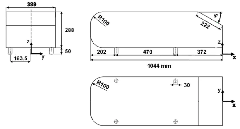
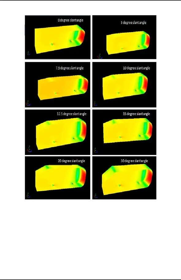
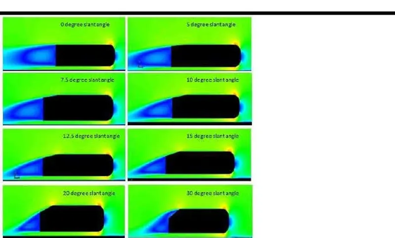
Variation of the slant angle (ψ) at the back of the geometry is the primary parameter in the characterization of the wake region. It has been found out that ψ = 30 deg is the critical value of slant angle. For Ahmed bodies, whose ψ is below 30 deg, a pair of counter-rotating vortices is generated. These vortices help in preventing the separation of flow along the slant surface. Above a ψ of 30, separation of flow occurs somewhere along the slant, and flow develops into a relatively larger recirculating region in the wake.

In this challenge, the study is performed on the Ahmed body whose slant angle is 20 degrees using Ansys fluent. The freestream speed of flow is taken as 25 m/s and the fluid is 'air'. The wake region is analyzed with contours and vector plots of velocity at certain probe locations behind the geometry. Parameters such as coefficient of lift, coefficient of drag, and point of separation of flow are estimated. Shown below is the CAD Model of the Ahmed body used in the challenge.

Negative pressure in the wake region

When the air moving over the vehicle is separated at the rear end, it leaves a large low-pressure turbulent region behind the vehicle which is known as the wake. This contributes to the formation of pressure drag which affects the vehicle performance.

When the vehicle is moving at a certain velocity the fluid imparts viscous force to the vehicle as long as it is in the viscous sublayer of the boundary. When the fluid reaches the rear end of the vehicle it gets detached from the surface of the body causing negative pressure in the wake region. The movement of the fluid around the vehicles depends on the geometry of the car and the Reynolds number.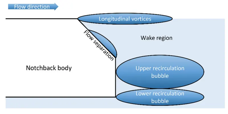

Modeling approach

Baseline simulation approach using k−εk-ε model.

• Ahmed's body is loaded into the Space claim.
• A single enclosure is drawn across Ahmed's body.
• Now the geometry is loaded for meshing.
• A baseline simulation is set up with the default element size of Ansys (413.6 millimetres).
• A named selection is created for the enclosure viz; inlet, outlet, symmetry.
• To create the named selection for the car the enclosure faces are hidden and box select is selected from the meshing toolbar and (car wall) name is given to it.
• Ansys Fluent window is opened and the geometry is loaded.
• Steady-state, the density-based solver is selected.
• Reference values are updated as per the prescribed conditions.
• In the inlet boundary condition, inlet velocity is 25 msecmsec and 300300 KK temperature are set.
• Drag-coefficient plot and lift-coefficient plot is created by setting the reference as (car walls).
• Hybrid initialization is selected.
• The solution is initialized by hitting t=0t=0.
• The cut-plane-z is created along Ahmed's body.
• The velocity contour, pressure contour is created along the cut-plane-z.
• The animation video is created for the velocity contour.
• The simulation is executed for 1000 iteration.

Simulation with a finer mesh using k−ωk-ωSSTSST.

• The first simulation ran successfully.
• The geometry is loaded into the SpaceClaim.
• The region of local refinement is created along Ahmed's body.
• As the body is perfectly symmetric, the simulation is executed by considering the only half body. This is the best practice where we can save on the number of cells and get the results faster as well.
• The geometry is loaded for meshing. The multizone method is selected for the outer enclosure to provide hexahedral mesh which provides accurate results in simulation.
• The element size for the first enclosure will vary as (100mm, 90mm, 80mm), the element size for the second enclosure will vary as (50mm, 45mm, 40mm), the element size of the leg of Ahmed's body will be 5mm, the first layer thickness, inflation layer, and the maximum thickness will be varied accordingly to imitate the experimental results.
• The rest procedure is the same as above, the necessary contour plot and graphs have been uploaded respectively.

Preprocessing and the solver settings

Case-1: External flow simulation over Ahmed body by creating a single closure and using default mesh value of ANSYS-FLUENT

Turbulence model: k−ε

Ahmed body model

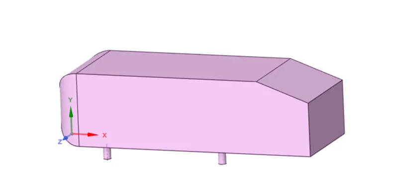
Creating an enclosure across Ahmed body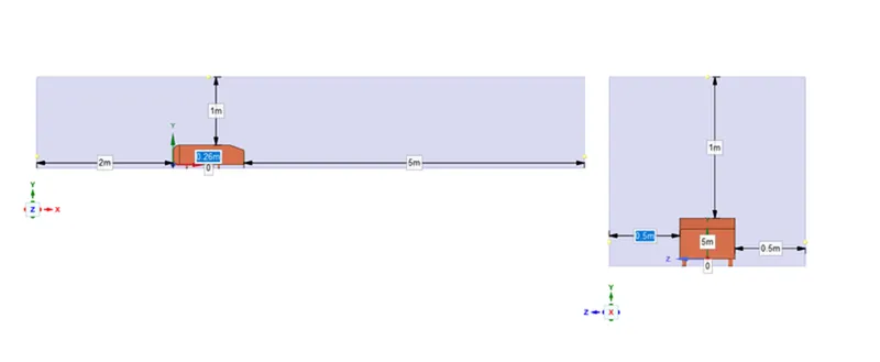

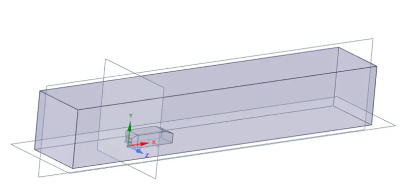
BODY ENCLOSE WITH PLANES

The three planes are normal to the x,y,z axes respectively.

As the body is perfectly symmetric, we can simulate by considering only half the body. This is the best practice where we can save on the number of cells and get the results faster as well.

To get half of Ahmed's body, the section mode is selected in SpaceClaim and the front view plain is selected to yield the desired result accordingly.

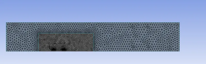
• Next, the mesh module is opened. Since the geometry of the outer enclosure is made of straight lines, the 'hex' mesh is used. The inner enclosure holds the surface of the Ahmed body and hence is 'triangle dominant'. The 'Multizone' mesh method is applied to the outer enclosure to connect between different mesh types. The base mesh size is set to 0.1 meters.
• The inner enclosure is given 'mesh body sizing' and is set to a size of 0.03 meters. Mesh 'face sizing' with a size of 0.004 meters is given on the cylindrical stands of the Ahmed body to prevent geometry distortion at the stands. To capture the near-wall physics accurately, a boundary layer mesh (Body fitted Mesh) (or) Mesh inflation is provided to the geometry. To come up with the right mesh size, the following calculations are done. Shown below is the mesh obtained.
• 

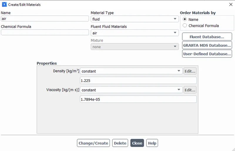
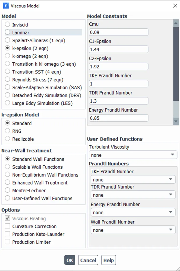
  Hybrid initialization is selected and the solution is initialized by hitting tt==00

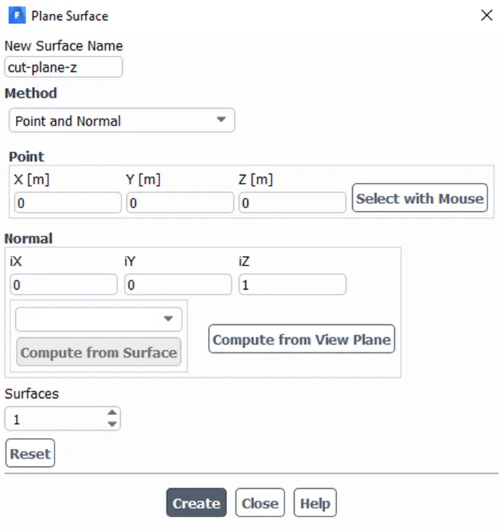
  Creating a cut plane to see the velocity change along Ahmed's body.

  Results

  Residual plot

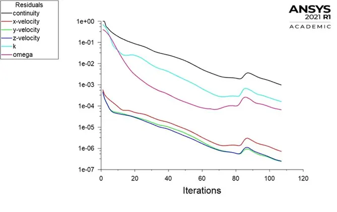
  • The number of iterations was set to 500.
  • But it is observed that the residuals have fallen below the specified tolerances and the solution attains convergence in ~110 iterations.
  • B) Coefficient of Drag and Coefficient of Lift:
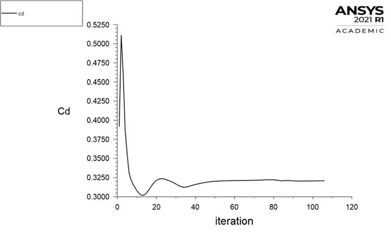
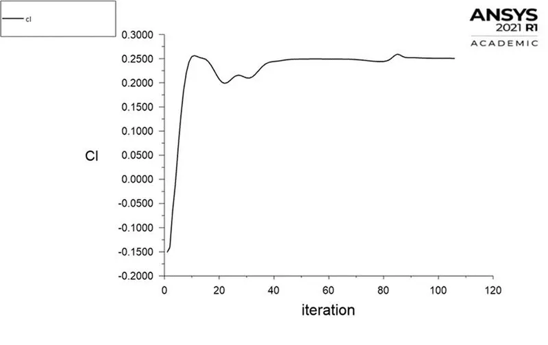
    • The formation of the low-pressure wake region dictates how high is the drag coefficient. The steady-state drag coefficient is found to be 32096. This result can be validated from [3] with an error of 7.34%.
    • The formation of vortices in the wake results in the lift. The steady-state lift coefficient is found to be 2504.
    1. C) Wall shear stress and the Point of separation:

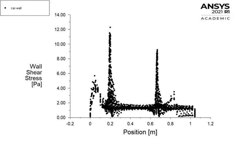
• Boundary layer separation occurs when there is an adverse pressure gradient and zero normal velocity gradient at the wall (i.e zero wall shear stress) simultaneously. The possibility of this occurring in the Ahmed body is at the slant surface.
• But, from literature, it is known that the flow does not separate at slant angles less than 30.
• The LHS plot is the wall shear stress plot along the entire length of the Ahmed body. The plot on the RHS is the zoomed-in range of the wall shear stress close to zero ranging from 0.0 Pa to 0.2 Pa.
• The result obtained is in accordance with the literature. The minimum wall shear stress obtained along the surface of the entire surface is always greater than 0.1.
• However, the flow separation occurs right at the end of the slant surface at the rear of the geometry. This flow separation results in a recirculation region of low pressure and determines the coefficient of drag of the body.

• D) X-Y Contours of Pressure and Velocity:
• 
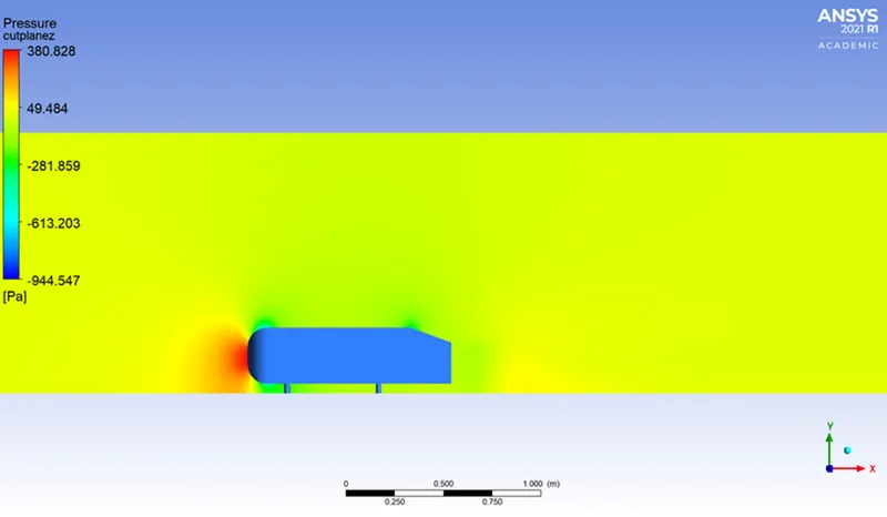
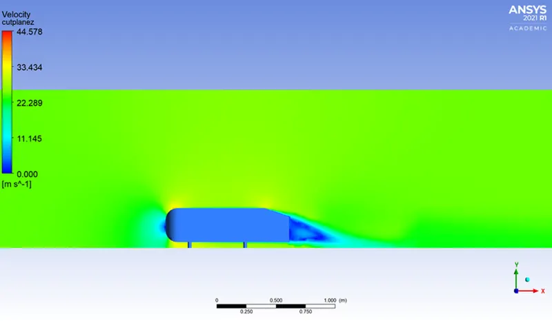
  • The contours are generated on an X-Y plane at Z = 0.
  • Just behind the slanted surface of the Ahmed body, a recirculation region is formed. This will be demonstrated more clearly by the vector plots in the coming section. The recirculation region has a lower pressure core and is represented by the light green patches in the contour. The scale defined in the contour represents the gauge pressureand hence shows negative pressure values at the recirculation region.
  • The pressure is maximum at the leading boundary of the Ahmed body because the flow is stagnated here. Also, at points where there exists curvature such as the filleted region at the leading boundary and the sharp beginning of the slant, there exist local low-pressure regions due to a sudden change in the geometry.
  • The velocity contour shows the flow over the slanted region. The flow does separate till the end of the slanted surface, after which separation occurs. A low-velocity region is formed at the recirculation region. This low-pressure region extends far into the wake of the car along with the formation of counter-rotating vortices that is shown in the next section.
  • At the different curvatures on the surface of the Ahmed body, where local low pressure exists, the regions have relatively higher velocities.
  1. E) Streamline and Vector Plots:
  2. a) Streamline:The Ahmed body is colored by the pressure and the streamlines are colored by velocity.
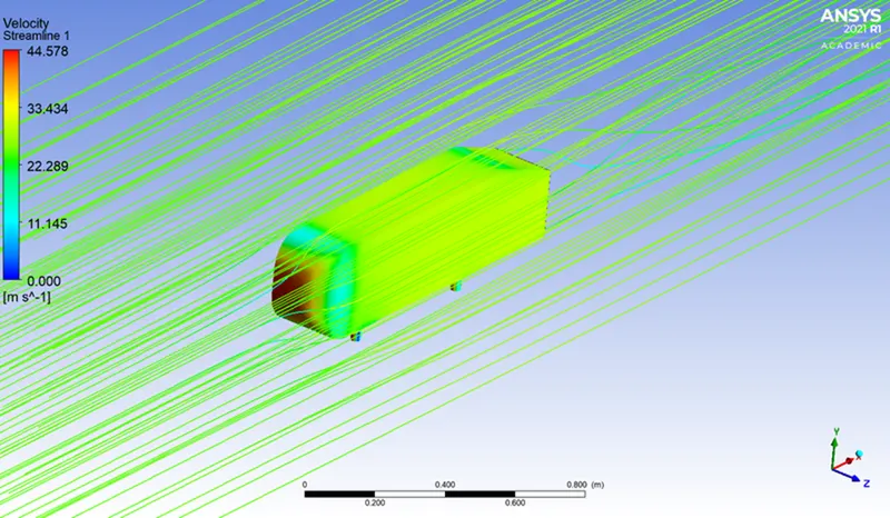
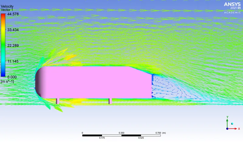
     • The vector plot shows the direction of flow at all locations. It is colored by velocity. The recirculation region is clearly seen from the images shown above.
     • This recirculation region further develops into a pair of counter-rotating trailing vortices that have a low-pressure region in the core. These vortices are visualized better in the next section.

     Grid Independence Test:

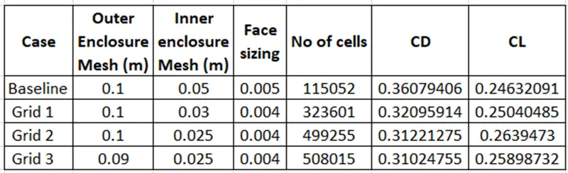
     The case is set up using meshes of increasing local refinement in an attempt to get mesh-independent results. The following are the results obtained for the combination of different mesh sizes. The maximum number of cells that can be used in the academic version of fluent is 512000 cells.

     The coefficient of drag attains a consistent value up to the 2nd decimal place in grid 2 and grid 3. Grid 3 holds the maximum refinement and the cell count is close to the maximum value. The error in the drag coefficient obtained using grid 3 with reference to [3] is 3.76%. Grid 2 produces an error of 4.41%. Hence, grid 3 and grid 4, both produce close values and both these results can be considered grid-independent. The results obtained in the other sections of the challenge are based on Grid 1. The meshes are shown below: