Week 3 - External flow simulation over an Ahmed body.

AIM-:
Study of Flow and Turbulence Structures in the Wake of a Simplified Car Model (Ahmed Model).

Objective: To perform external flow simulation over an Ahmed body.

The expected results will include:

1. Velocity and pressure contours.

2. The drag coefficient plot for a refined case. ( For a velocity of 25m/sec, the drag coefficient should be around 0.33).

3. The vector plot clearly showing the wake region.

4. Perform the grid independence test and provide the values of drag and lift with each case.

Theory-:
Ahmed Body:

The Ahmed Body was first created by S.R. Ahmed in his research “Some Salient Features of the Time-Averaged Ground Vehicle Wake” in 1984. Since then, it has become a benchmark for aerodynamic simulation tools.

Ahmed body is a bluff body that represents a generic car body. It has a simplistic shape and has the basic aerodynamic properties of a vehicle and has been used as a reference in many aerodynamic studies. so, Ahmed body shape is simple enough to model.

Importance of Ahmed body:

The three-dimensional flow around a vehicle has become a subject of significant importance in the automotive industry. One apparent technique of improving the fuel efficiency of a vehicles is to reduce aerodynamic drag force by optimizing the body shape. Execution of fine aerodynamic design under stylistic constraints requires an immense understanding of the flow pattern phenomena and, especially, how the aerodynamics are impacted by changes in body shape. The flow area which is presents the major contribution to a cars drag is the wake flow backing the vehicle. The point at which the flow separates directs the size of the separation zone, and as a result the drag force. Clearly, a more accurate simulation of the wake flow

Most cars have an average drag coefficient of between .30 and .35. Boxy cars have a higher number, like the HUMMER® H2 vehicle at .57, while more streamlined and agile cars have a lower number, like the Mercedes-Benz® C-Class® vehicle at .24. Again, this is just an average measurement. The exact drag coefficient of a car varies with the Reynolds number and various other factors.

Drag Coefficient:

The drag coefficient quantifies the resistance of an object in a fluid environment. It is not an absolute constant for a body’s shape because it varies with the speed and direction of flow, object shape and size, and the density and viscosity of the fluid.
The lower the drag coefficient of an object, the less aerodynamic or hydrodynamic drag occurs. In terms of a car, the lower the drag coefficient, the more efficient the car is. As well as affecting the top speed of a vehicle, the drag coefficient also affects the handling. Cars with a low drag coefficient are sought after, but decreasing the drag drastically can reduce the downforce and lead to loss in road traction and a higher chance of car accidents.

Cd=2⋅Fdρ⋅V2⋅A

where, Cd= Drag coefficient

Fd= Drag force

ρ= Density

A= Area

V= Velocity

Negative Pressure at wake:

When the vehicle is moving at a certain velocity, the viscous effects in the fluid are restricted to a thin layer called boundary layer (Outside the boundary layer is the inviscid flow). As thousands and even millions of air molecules draw near the car’s front, they start compressing, thus raising the air pressure on the front of the vehicle. Likewise, the air molecules that are travelling along the car’s sides are at atmospheric pressure. This means the pressure is lower than the molecules on the vehicles front. i.e. the fluid flow imposes pressure force on the boundary layer. When the air reaches the rear part of the vehicle, the fluid gets detached. Within the boundary layer, the movement of the fluid is totally governed by the viscous effects of the fluid. The fluid moving around the vehicle is dependent on the shape of the vehicle and the Reynolds number.

There is another important phenomenon, which affects the flow of the car and the performance of the vehicle. This phenomenon is commonly known as Wake of the vehicle. When the air moving over the vehicle is separated at the rear end, it leaves a large low-pressure turbulent region (vacuum) behind the vehicle known as the wake. This wake contributes to the formation of pressure drag, which is eventually reduces the vehicle performance.

Flow Seperation :

Whenever there is relative movement between a fluid and a solid surface, whether externally round a body, or internally in an enclosed passage, a boundary layer exists with viscous forces present in the layer of fluid close to the surface. Boundary layers can be either laminar or turbulent. A reasonable assessment of whether the boundary layer will be laminar or turbulent can be made by calculating the Reynolds number of the local flow conditions.

Flow separation or boundary layer separation is the detachment of a boundary layer from a surface into a wake. Separation occurs in flow that is slowing down, with pressure increasing, after passing the thickest part of a streamline body or passing through a widening passage, for example. Flowing against an increasing pressure is known as flowing in an adverse pressure gradient. The boundary layer separates when it has travelled far enough in an adverse pressure gradient that the speed of the boundary layer relative to the surface has stopped and reversed direction. The flow becomes detached from the surface, and instead takes the forms of eddies and vortices.

Y⁺ Concept :

It's important that your mesh near the wall is properly sized to ensure accurate simulation of the flow field. The y+ value is a non-dimensional term that can be used to understand how coarse or fine our grid is.

with a desired y+ value, we can calculate the wall distance or first cell height (y).

Re=ρ⋅V⋅Lμ

Cf=0.026Re17

Tw=Cf⋅ρ⋅V22

Uf=√Twallρ

y=y+⋅μUf⋅ρ

Where ,

ρ , µ are fluid density and viscosity ;

U is the free stream velocity ;

L is characteristic length ;

U_τ is frictional velocity ;

τ_ω is wall stress , C_f is skin friction coefficient

In this case , we take Y⁺=200 ;

From the calculation ,

We got first layer thickness is found to be 3 mm(0.003m)

Thus , Total thickness =3 * (1.2)^(6-1) =7.4645 mm ≈ 7.5 mm

PROCEDURE :

The geometry can be imported from another CAD software or it can be created in ANSYS. I imported a .STEP file for this project in SpaceClaim.

Since this is a complex simulation and the ahmed body is symmetrical along the z axis, the geometry was split into two along the z axis using ANSYS's split tool.

This is the geometry after the spliting:

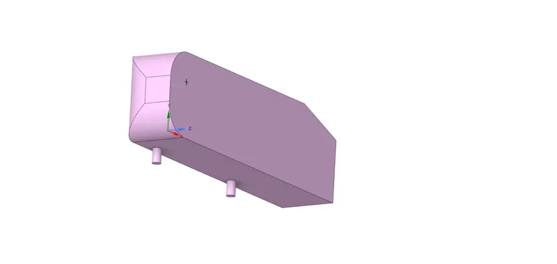
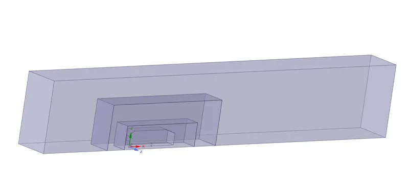
A wind tunnel has to be created around the ahmed body, there are multiple methods to achieve this, but the easiest is using the enclosure tool in ANSYS to generate the tunnel. The inlet of the wind tunnel is 2 metres from the front of the ahmed body, the outlet is 5 metres from the back of the body. The height and of the enclousure is 1 metre above the ahmed body while the width is 0.5m from the side of the body. The enclousure is checked for Interference and it is repaired as well.

Further enclousures may be created for mesh refinement.

This is the final geometry with three enclousures:

Make sure the original extrusion is suppressed before closing SpaceClaim.

Meshing:

The base size is 0.1m. There are multiple mesh controls used to generate the mesh for this geometry, they are:

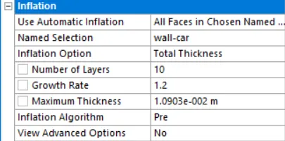
1. Mesh -> Inflation:

This option is used to accurately capture the boundary layers on the surface of the body.

An inlet velocity of 25m/s, the wall spacing is 0.42mm. ie. The size of the element on the ahmed body should be 0.42mm high. If the initial thickness is 0.42mm, number of layers are 10 for a growth rate of 1.2 => the total thickness is 10.903mm (recall geometric progession)

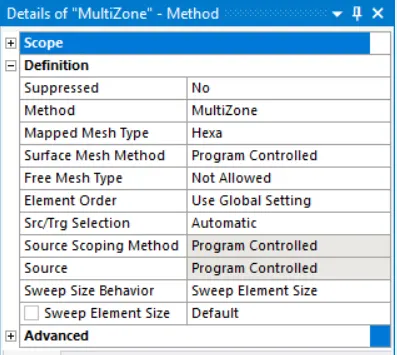
2. Method -> Multizone:

This option is used to generate mesh in the outer region which is primarily hexahedral

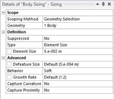
3. Sizing -> Body Sizing:

This option is used to refine the larger inner enclousure of the wind tunnel. The increased size gives us more accurate results near the ahmed body. Element size is 0.05m.

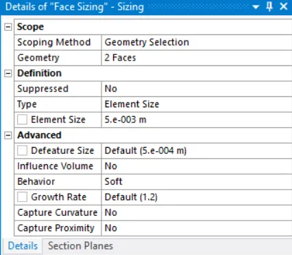
4. Sizing -> Face Sizing:

This method is used to ensure that the legs of the ahmed body are circular and not polyhedral.

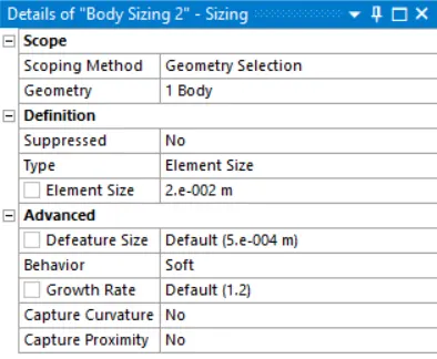
5. Sizing -> Body Sizing:

This option is used to refine the smaller inner enclousure of the wind tunnel. The increased size gives us more accurate results near the wake region. Element size is 0.02m.

After all these controls are applied, this is the resultant base mesh:

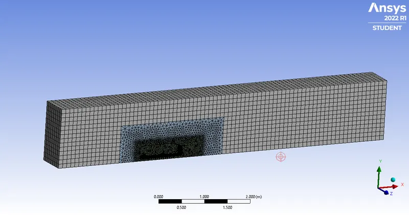
Zooming in,

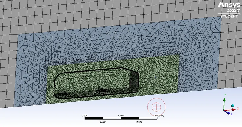
These are the mesh metrics:

As seen, most elements have their quality >0.6, hence it can be said that the mesh quality is satisfactory.

Setup:

Boundaries

inlet - inlet

outlet - pressure outlet

wall-car - wall (no-slip)

back, top and bottom - symmetry

symmetry zplane - symmetry

A separate boundary was created for the symmetry plane to make post processing easier.

Reference Values

The most important values here are: Area, Density, Length and Velocity.

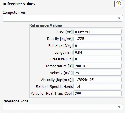
The area was calculated using ANSYS Fluent, Results -> Reports -> Projected Areas:

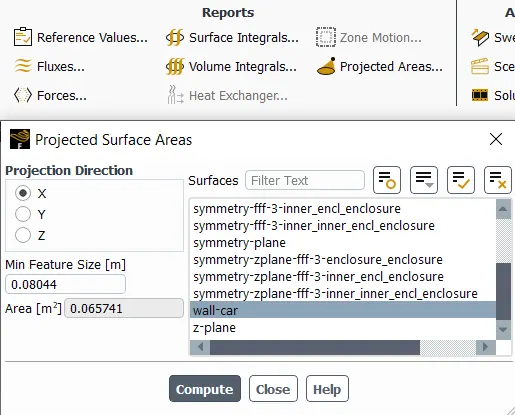
This is the cross sectional area for the half ahmed body

k-omega SST was used for all simulations for this project due to its excellence in solving external flows and wake regions.

Reports

Two reports were created.

1. Lift Coefficient of wall-car

2. Drag Coefficient of wall-car

Solution - Methods

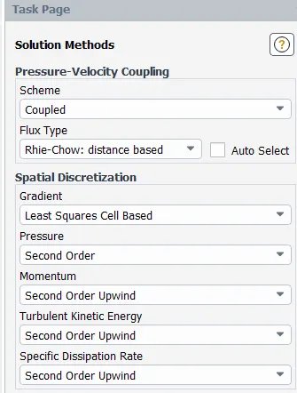
Simulation of the base setup

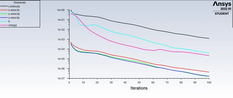
The simulation ran for 100 iterations and the results are below:

Residuals

Drag Coefficient:

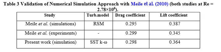
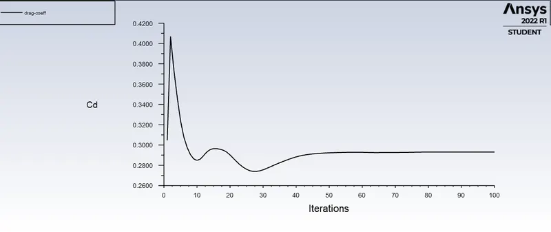
The final value of drag coefficient is 0.29310978, which is in agreement with experimental and simulation data.

Lift Coefficient:

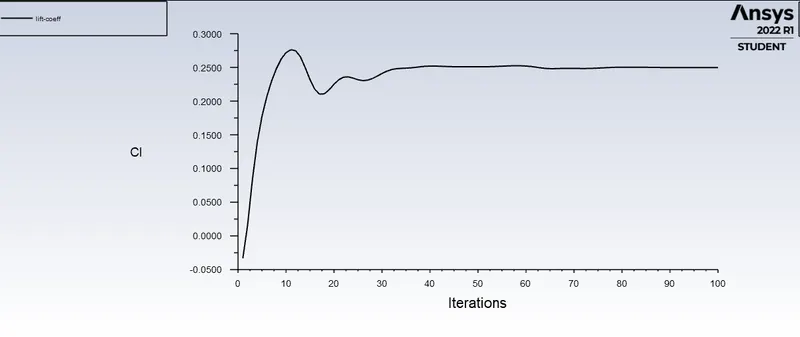
The final value of lift coefficient is 0.24969179, the discrepancy is due to variation in reynold's number and low mesh resolution near some regions of the ahmed body.

Contours, Plots and Vectors

Note: All plots, contours and vectors were obtained from the finer mesh, due to its higher solution clarity.

1. Velocity contours:

These were taken in CFD - Post.

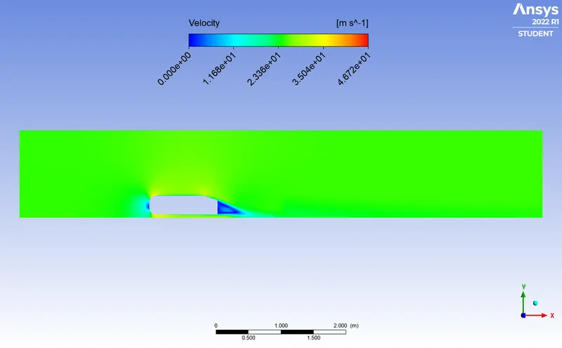
Zooming in,

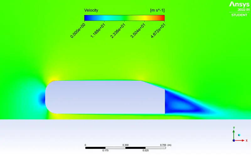
Zooming in further,

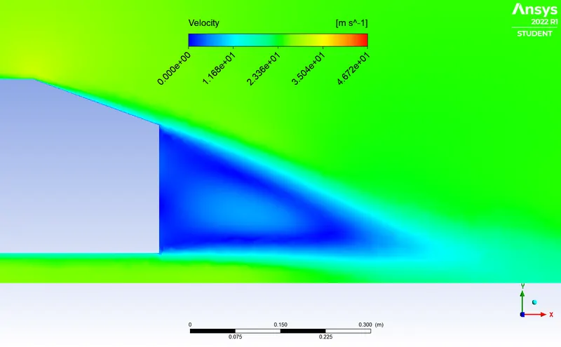
The wake is clearly visible.

2. Pressure Contour:

These were taken in CFD - Post.

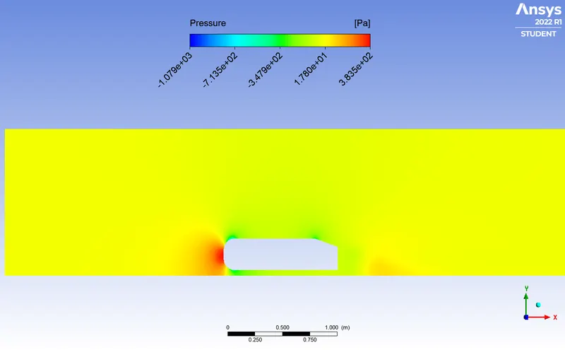
Zooming in,

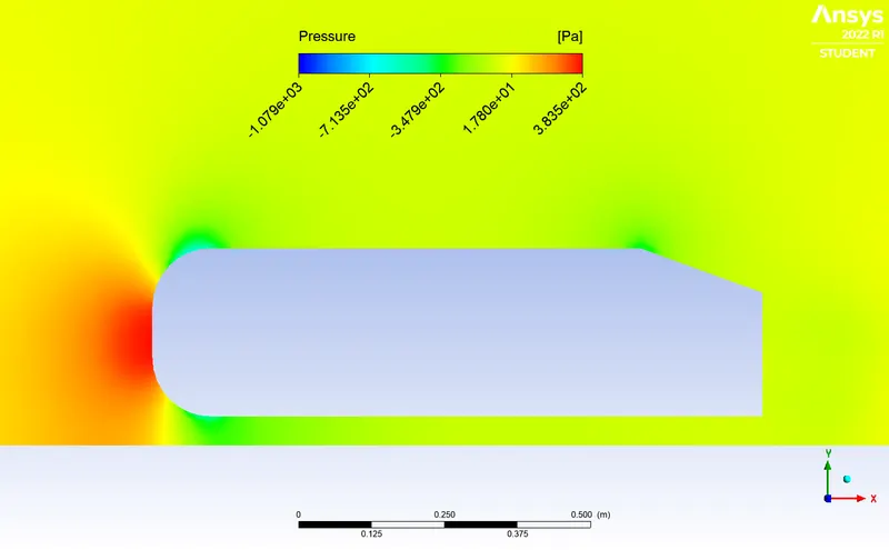
There is a high pressure region at the front of the body due to how flowing air is acculumated at the front.

The pressure is negative in some regions, this is not an error in the simulation but rather how ANSYS and Fluent functions. The "pressure" displayed in ANSYS is actually gauge pressure, the gauge pressure is 0 when the total pressure is the atmospheric pressure. In this case, the "pressure" being negative is merely the pressure dropping below atmospheric in some regions.

3. Vector Plot:

These were taken in CFD - Post. The background contour is the velocity contour.

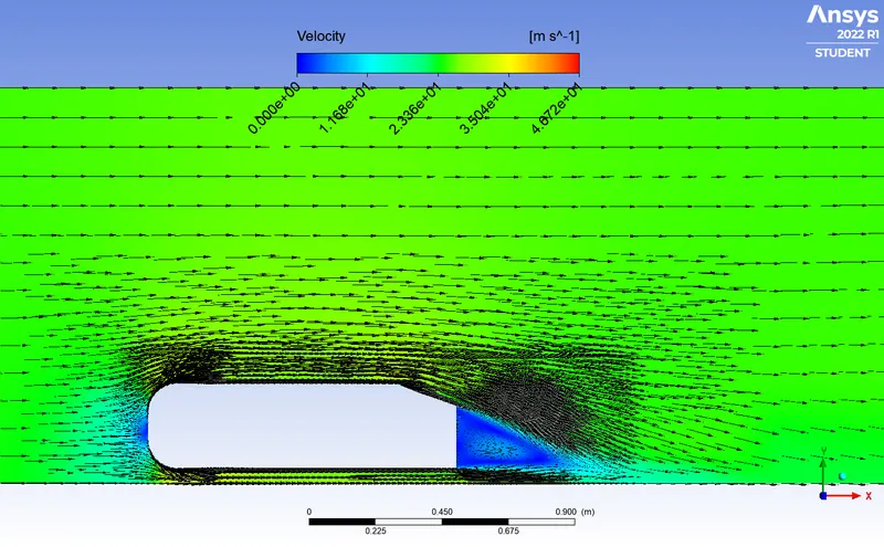
Zooming in,

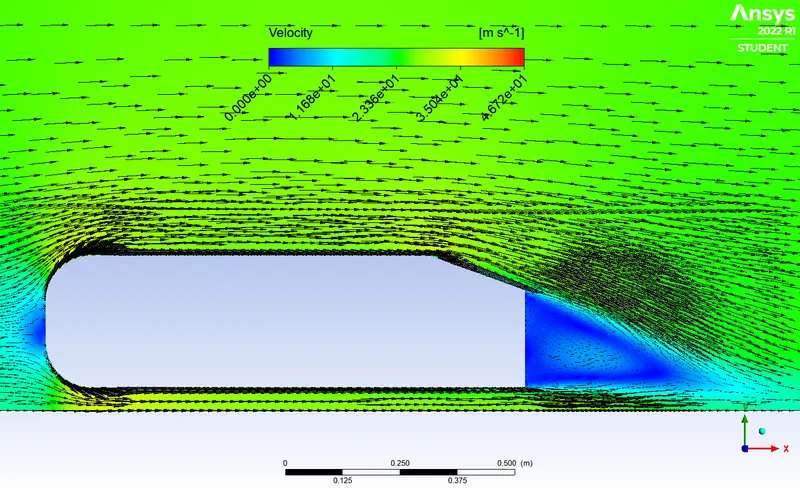
Zooming in further near the wake region,

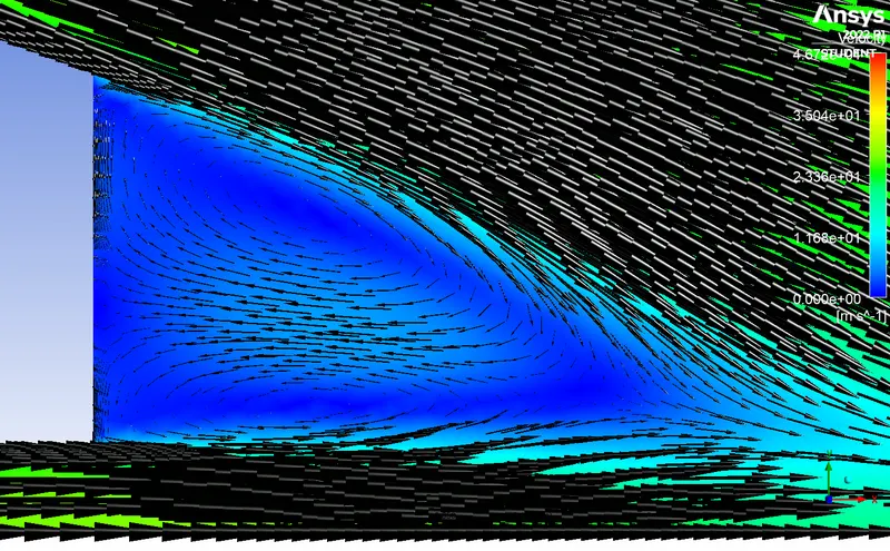
Switching the type of arrow to see the lines more clearly,

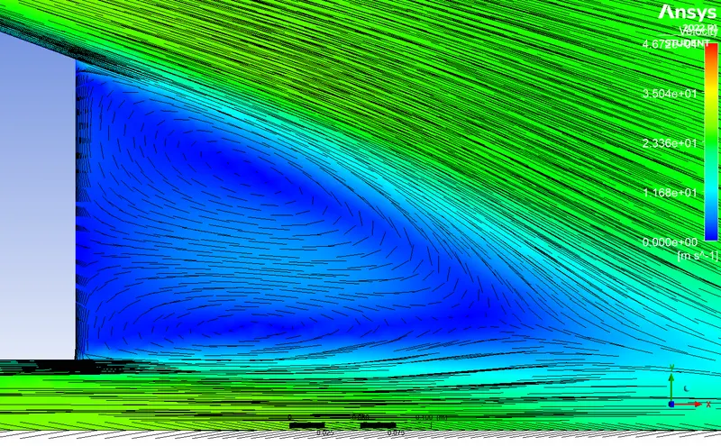
Two distinct regions can be spotted behind the ahmed body with two vortices (seen from this view) or recirculating regions behind the ahmed body.

Initially the wake regions has some disturbances but they are eventually ironed out the solution reaches steady state.

Grid Dependence Test

A Grid Dependence Test is used to ascertain whether the final values of the solution are dependent on the mesh or not. This is an important test to ensure the simulation results are correct.

In this test, the test will involve 2 different simulations - one where the mesh becomes more finer and other where the mesh becomes more coarser.

Coarser Mesh:

For this test, the smaller inner enclousure is removed (point 5 under Meshing) and the simulation is ran for the same parameters.

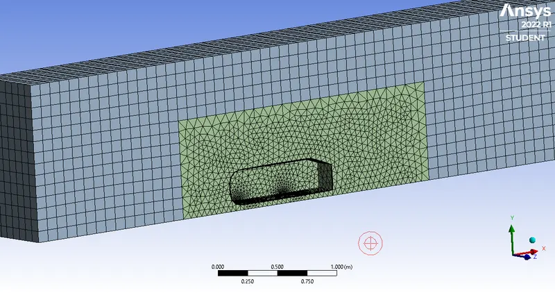
These are mesh statistics:

The values of drag and lift coefficient are below:

Lift Coefficient: 0.22592755

Drag Coefficient: 0.35537949

Finer Mesh

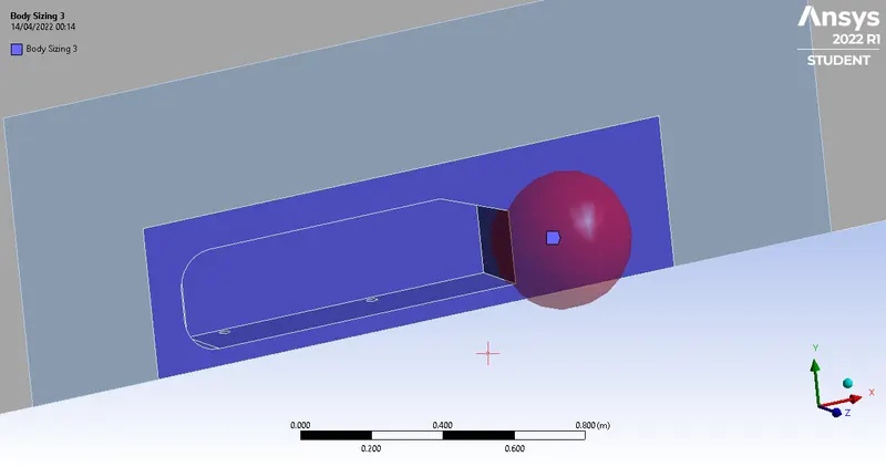
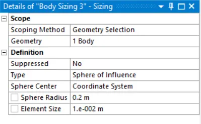
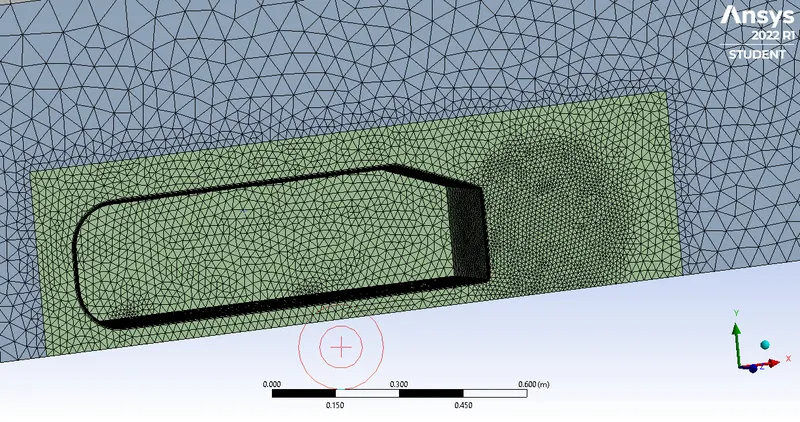
For this test, a spherical region centered at x=1.2, y=0.1 and z=0 is created and the mesh size in this region is decreased.

It was added going to Mesh -> Controls -> Sizing

This is the region seen in ANSYS:

The details of the regions are below:

This is the resultant mesh seen in ANSYS:

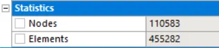
These are mesh statistics:

Other simulation parameters were kept the same as the baseline simulation and the simulation was ran:

The values of drag and lift coefficient are below:

Lift Coefficient: 0.22918563

Drag Coefficient: 0.28130557

Summary of Grid Dependence Test

	Lift Coefficient	Drag Coefficient	Nodes	Elements
Coarser Mesh	0.22592755	0.35537949	37033	104163
Base Mesh	0.24969179	0.29310978	83137	309948
Finer Mesh	0.22918563	0.28130557	110583	455282

Conclusion

• It can be inferred that the grid independence test is performed to know the smaller cell size for convergence.
• Apart from mesh refinement, convergence depends on the Y+ value, inflation layer, it is advisable to use k-ωSST as the turbulence value because it calculates the values well near the wall.
• As the setup is refined drag coefficient, lift coefficient decreases.
• Y+ plays an important role in determining the value of drag.
• The negative pressure in the wake region is primarily because there is no flow in that region. This can be further attributed to various factors such as separation and recirculation which is evident from the vector plot near the wake region.
• The point of separation occurs at the rear end of the vehicle, the separation occurs beyond this point where it can be observed that the flow recirculates and attaches it to the boundary layer.