Week 3 - External flow simulation over an Ahmed body.
Simulation of Airflow around Ahmed Body
- Objective
- To make 3d model of Ahmed Body and mesh it.
- To solve the model and calculate coefficient of drag and coefficient of lift.
- To generate pressure, velocity contour and vector plot.
- To perform grid independence test.
- Introduction
Computational fluid dynamics is a branch of fluid mechanics in which fluid slow is analyzed using numerical methods. There are many types of CFD software available on the market and Ansys fluent is one of them. CFD simulations is an efficient tool in automatic industry used extensively for design. This allows the designers to obtain a quick and proper analysis before going ahead to the final step. CFD analysis in the car industry is used in the determination of the applied forces and that of the vehicles wake during moving. CFD also is used to analyze the effect of wake on the vehicle’s efficiency and capability in comparison with other cars.
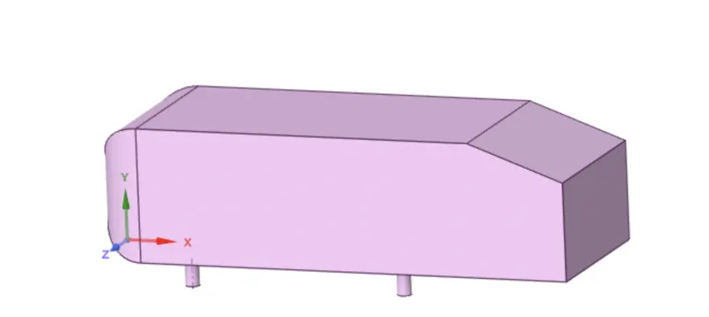
In this study we will perform simulation on Ahmed body. Ahmed Car Body is the standard model that can be used as validating case, in industry and CFD simulation Ahmed Body is a generic car-type bluff body with a slant back has different angles from 0 – 40 degrees.
- Theory
One major area of study in the automotive industry is the study of air flow over a car and its resultant drag and lift forces. High drag force will cause a reduction in fuel efficiency and a vehicles top speed, whilst lift can positively or negatively affect tire traction depending on whether it is in an upwards or downwards direction. (Costa, B 2015) Accurate measuring of the drag and lift forces computationally in turn depends on accurate modelling of turbulent flow, thus there is a need verify the accuracy of current turbulence models in an automotive context. The accurate modelling of turbulence has always been a considerable challenge for engineers throughout history. This fluctuating nature of turbulence makes a deterministic approach very difficult, so most current methods of solving turbulence related problems and modelling tend to be more approximating in nature.
A great deal of studies regarding airflow and turbulence behavior on a car involve the use of the Ahmed body, which was first devised by S, Ahmed in 1984. He said referred Ahmed body as a strong three-dimensional displacement flow in front, relatively uniform flow in the middle and a large structured wake at the rear. It has had a significant impact on research in the automotive industry, used to study and validate flow over an automotive in both wind tunnel and CFD environments. In the case of CFD its simple shape reduces required computational power and time taken to model the body and run simulations.
Ahmed body
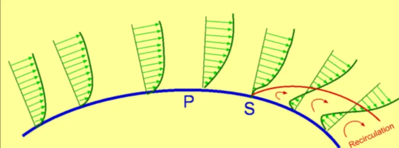
Point of separation and its significance – Flow separation is position where the boundary layer leaves the surface of the body in other words it is region where wall shear stress is zero.
Point of separation totally depends on the type of geometry. Pressure gradient is one the factor which affects fluid flow. Change in kinetic energy is directly linked to a change in static pressure according to Bernoulli principle. In this case, the increase in kinetic energy is at the expense of the pressure (energy). The static pressure thus decreases to a minimum up to the thickest point of the cylinder. The pressure gradient in x-direction is negative in this area.
Now the effective cross-section of the flow increases, as the cylinder cross-section decreases flow slows down and the static pressure rises again in the x-direction to finally reach the level of the atmosphere This pressure gradient acting against the actual direction of flow is called adverse pressure gradient and it is positive. Depending on the shape of the body, the resulting adverse pressure gradient can become very large due to the decrease in speed and the boundary layer thickness increases significantly. This will lead to a flow separation.
The point of separation plays a significant role in real world phenomenon especially in aerodynamics, where flow separation results in reduced lift and increase in drag and it causes buffeting of aircraft structure.
Flow separation phenomenon
Negative pressure in wake region
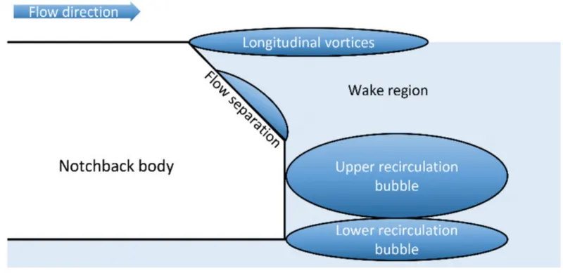
When the air moving over the vehicle is separated at the rear end, it leaves a large low-pressure turbulent region behind the vehicle which is known as the wake. This contributes to the formation of pressure drag which affects the vehicle performance.
When the vehicle is moving at a certain velocity the fluid imparts viscous force to the vehicle as long as it is in the viscous sublayer of the boundary. When the fluid reaches the rear end of the vehicle it gets detached from the surface of the body causing negative pressure in the wake region. The movement of the fluid around the vehicles depends on the geometry of the car and the Reynolds number.
4.Procedure
There are three main steps of any simulation: the first is pre-processing, which includes geometry setup, cleaning and mesh generation. The second step is solving the model and third one is post-processing which includes plotting, contour generation and analysis. In the study we proceeded with the following procedure and data values.
Modeling approach
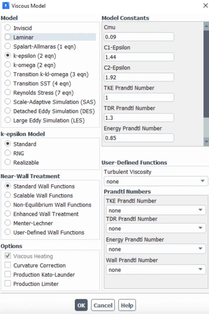
Baseline simulation approach using `k-epsilon` model.
Ahmed's body is loaded into the Space claim.
A single enclosure is drawn across Ahmed's body.
Now the geometry is loaded for meshing.
A baseline simulation is set up with the default element size of Ansys (413.6 millimeters).
A named selection is created for the enclosure viz; inlet, outlet, symmetry.
To create the named selection for the car the enclosure faces are hidden and box selection is selected from the meshing toolbar and (car wall) name is given to it.
Ansys Fluent window is opened and the geometry is loaded.
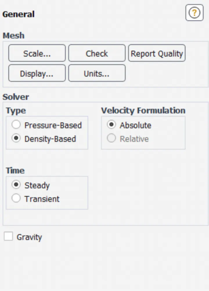
Steady-state, the density-based solver is selected.
Reference values are updated as per the prescribed conditions.
In the inlet boundary condition, inlet velocity is 25 `frac{m}{sec}` and `300` `K` temperature are set.
Drag-coefficient plot and lift-coefficient plot is created by setting the reference as (car walls).
Hybrid initialization is selected.
The solution is initialized by hitting `t=0`.
The cut-plane-z is created along Ahmed's body.
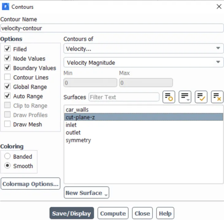
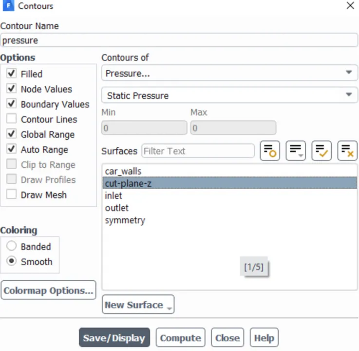
The velocity contour, pressure contour is created along the cut-plane-z.
The animation video is created for the velocity contour.
The simulation is executed for 1000 iterations.
Simulation with a finer mesh using `k-omega``SST`.
The first simulation ran successfully.
The geometry is loaded into the Space Claim.
The region of local refinement is created along Ahmed's body.
As the body is perfectly symmetric, the simulation is executed by considering only half the body. This is the best practice where we can save on the number of cells and get the results faster as well.
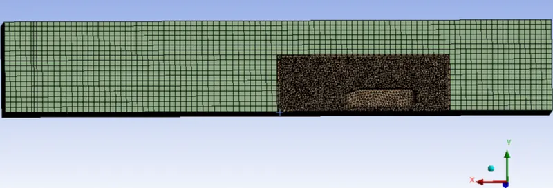
The geometry is loaded for meshing. The multizone method is selected for the outer enclosure to provide hexahedral mesh which provides accurate results in simulation.
The element size for the first enclosure will vary as (100mm, 90mm, 80mm), the element size for the second enclosure will vary as (50mm, 45mm, 40mm), the element size of the leg of Ahmed's body will be 5mm, the first layer thickness, inflation layer, and the maximum thickness will be varied accordingly to imitate the experimental results.
The rest of the procedure is the same as above, the necessary contour plot and graphs have been uploaded respectively.
Case/mesh parameters Case1 Case2 Case3
Element Size 0.1 0.115 0.130
Body element size 0.05 0.07 0.09
Face element size 0.01 0.01 0.01
Number of elements 104950 51594 29381
Preprocessing and the solver settings
Case-1: External flow simulation over Ahmed body by creating a single closure and using default mesh value of ANSYS-FLUENT
Turbulence model: `k-epsilon`
Ahmed body model
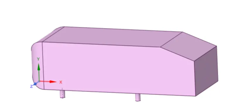
Creating an enclosure across Ahmed body
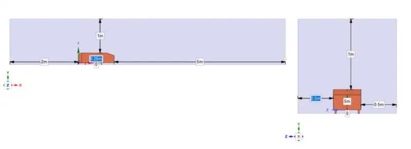
Creating a plane section on the origin
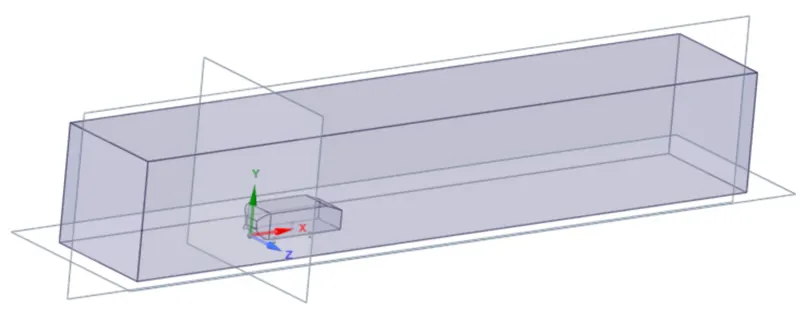
The three planes are normal to the x,y,z axes respectively.
As the body is perfectly symmetric, we can simulate by considering only half the body. This is the best practice where we can save on the number of cells and get the results faster as well.
To get half of Ahmed's body, the section mode is selected in Space Claim and the front view plain is selected to yield the desired result accordingly.
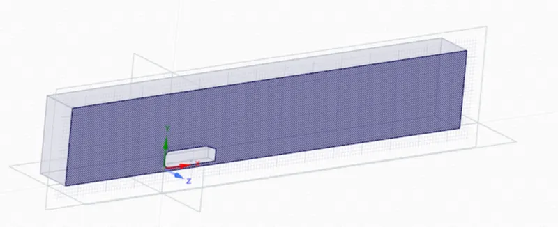
Once the geometry part is complete, it is loaded in the meshing window to perform the baseline meshing.
Simulating with a default mesh size of Ansys-Fluent
Creating named selection to set up physics and boundary conditions.
Inlet boundary condition (velocity inlet).
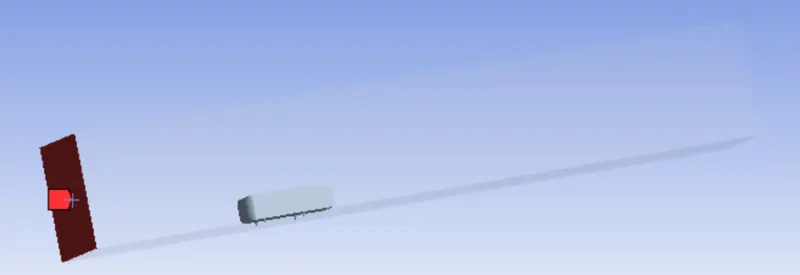
Outlet boundary condition (pressure outlet)
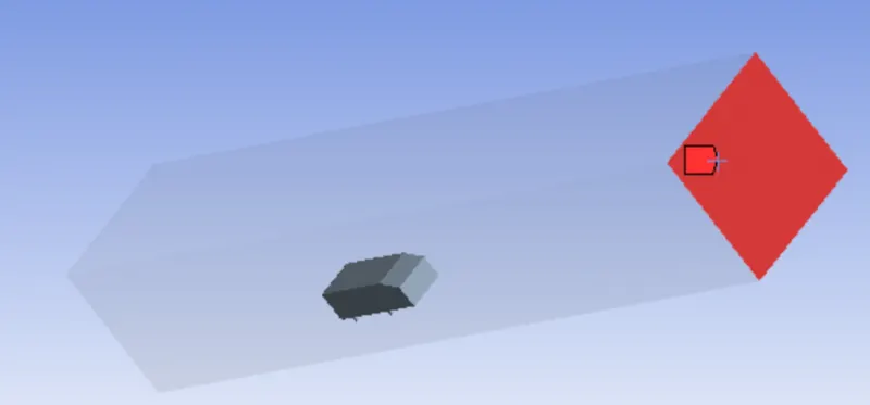
Symmetry boundary condition
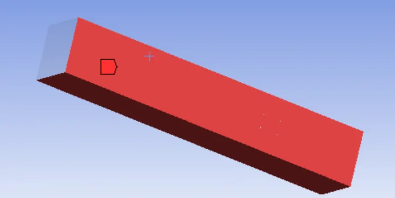
Creating named selection for car walls
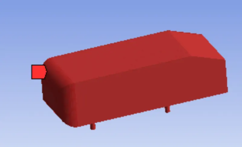
To create the named selection for car walls we need to hide the faces of the enclosure by hitting function key f8.
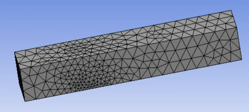
Performing meshing with default mesh size in ANSYS-FLUENT
Element size: `0.4136 m`
Number of elements: `83781`
The geometry is cut into two halves by using a section plane
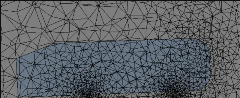
Thus, the mesh is created inside Ahmed's body which is not good for simulation because the flow outside Ahmed's body is taken into account. It can be fixed by going back to Space claim, one of the copies should be suppressed for physics.
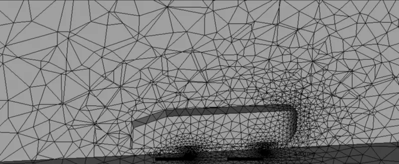
The required geometry is then loaded into the ANSYS-FLUENT window.
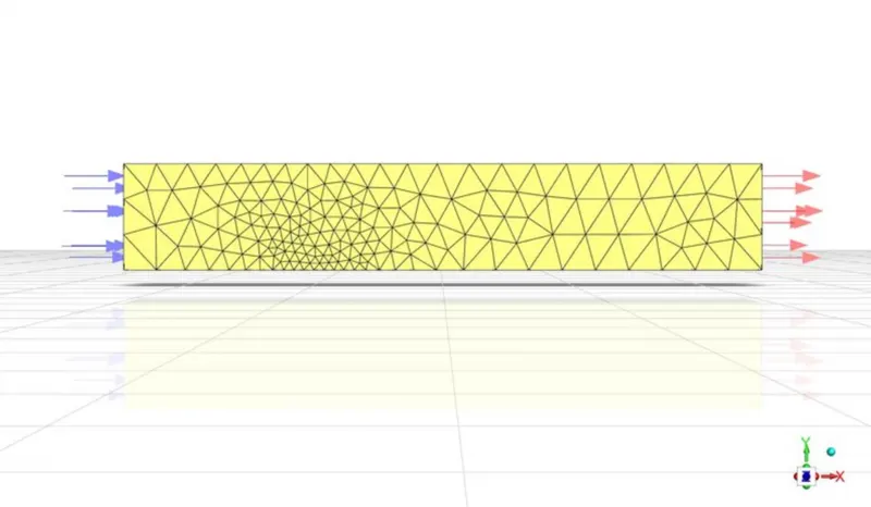
Simulation procedure
Setting up of physics
Reference values
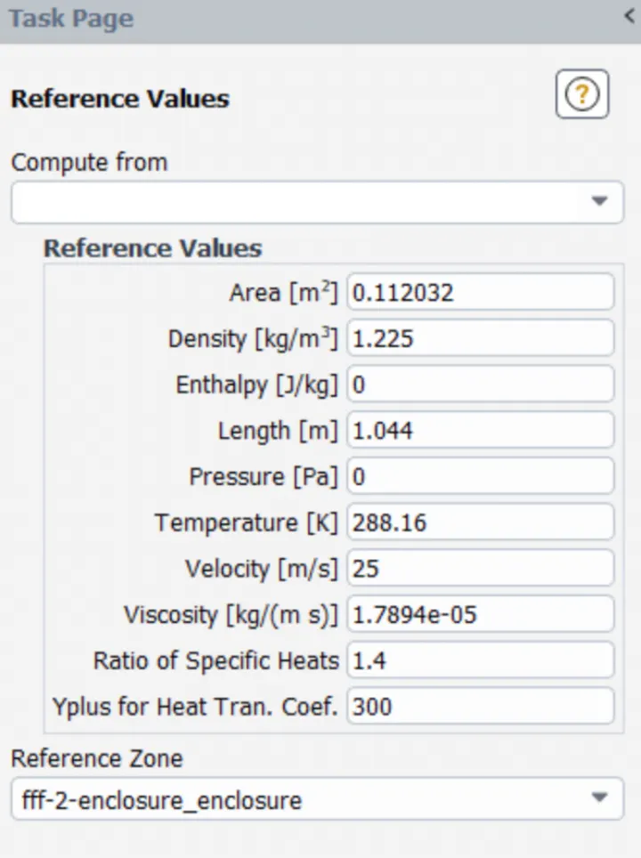
The frontal area of Ahmed body
Area `=``0.389***0.1635``=``0.112032``m^2`
Length of Ahmed's body `=``1.044``m`
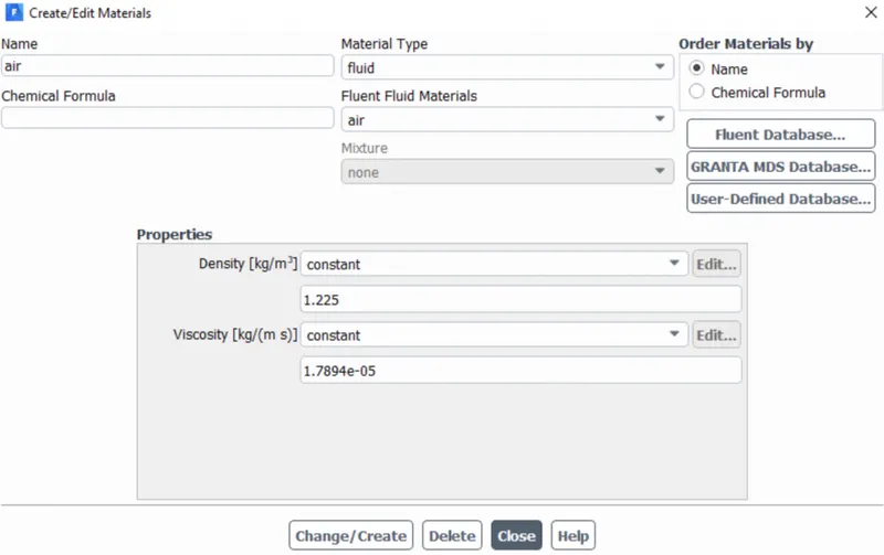
Material properties
Viscous model
Hybrid initialization is selected and the solution is initialized by hitting `t``=``0`
Creating a cut plane to see the velocity change along Ahmed's body.
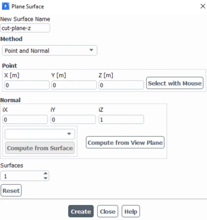
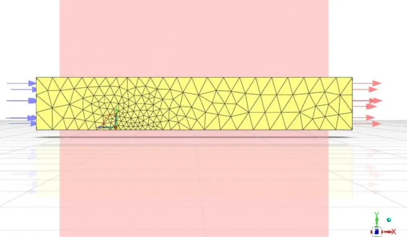
Creating contour plot along cut plane z
Results
Residual plot
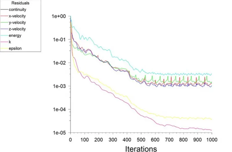
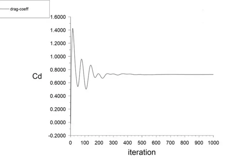
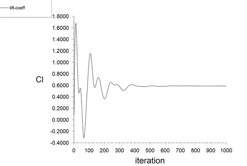
After 700 iterations, the same repeating trends are observed.
Drag-coefficient plot
Lift-coefficient plot
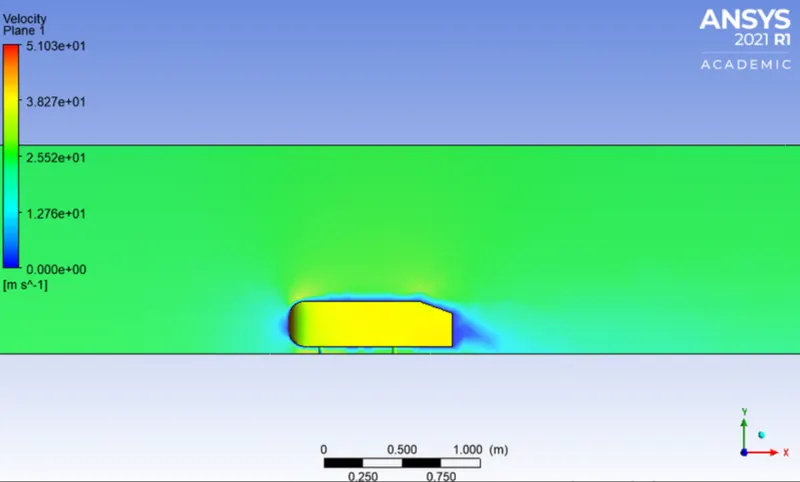
Velocity contour
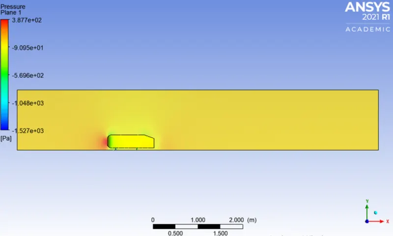
Pressure contour
Drag-coefficient 0.7253
Lift-coefficient 0.5865
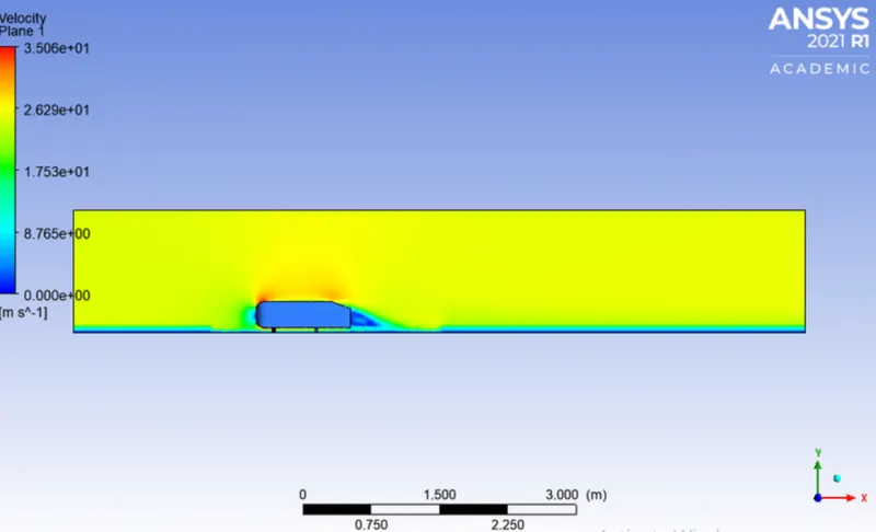
It can be inferred from the following figure that the results of the base simulation are distorted and do not capture the turbulent flow behind the body perfectly. This simulation captures the wake length, high velocity, low-velocity areas which can be used to further refine the mesh value around the Ahmed body and add a local refinement around.
Case-2 (a) External flow simulation over Ahmed body with finer mesh in a double enclosure.
Turbulence model: `k-omega` `SST`.
First refinement
A region of local refinement is added to the Ahmed body.
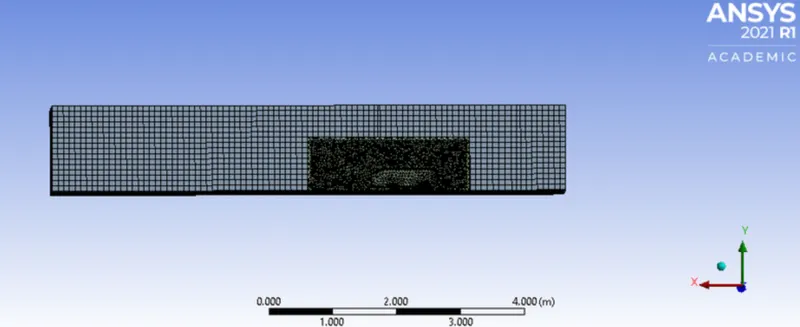
Share Topology: It is set to share. It is used for sharing the information between the two enclosures and also to make the mesh uniform.
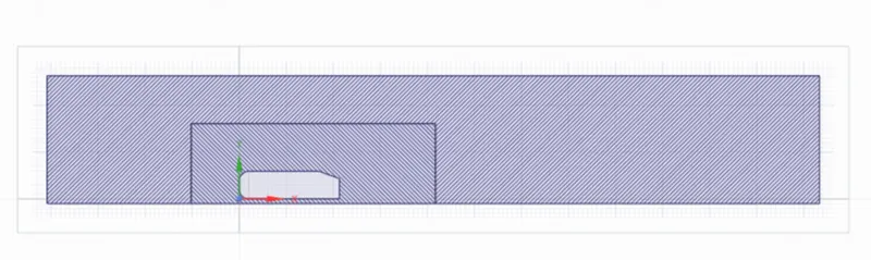
The geometry is loaded into the meshing window.
Meshing
The meshing involves the following steps
Method
Outside the box, the hexahedral mesh is used. The mesh is of the highest quality and gives higher accuracy.
Multizone method: It is used to create hexahedral meshes wherever possible and for other regions where different mesh types are used it will connect properly.
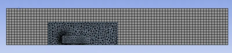
Sizing: It is defined as increasing the number of elements by decreasing the element size. The element size of the second closure is `0.05``m`
Element size for the first enclosure: `100``mm` or `0.1``m`
Maximum size for the first enclosure: `100``mm` or `0.1``m`
Element size for the second enclosure: `50``mm`
Element size of pillars of Ahmed body: `5``mm`
Number of elements: 1,92,628
Inflation layer: It is the process of adding layers to the boundary to cover the boundary layer thickness fully.
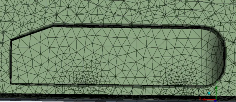
The first cell height predicted value is `5` `mm`
Inflation layer: `5`
Last layer thickness: `15` `mm`
Y+ value: 345
Residual plot
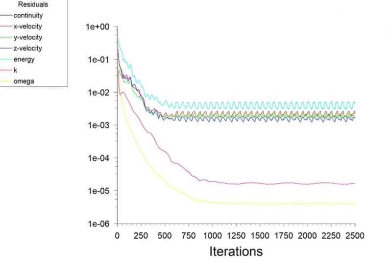
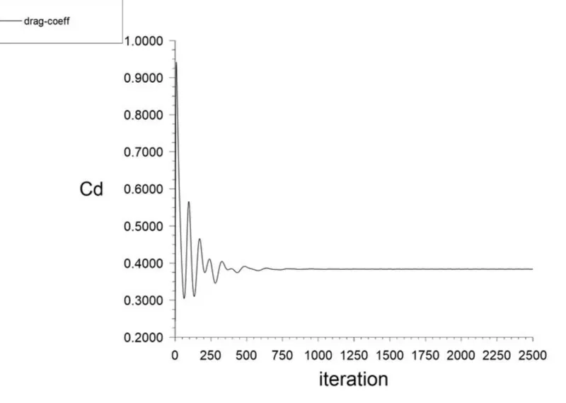
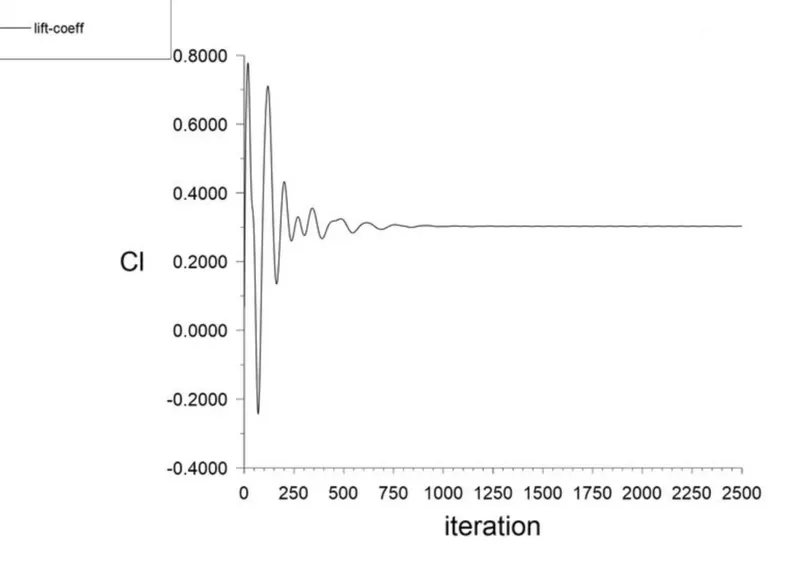
After 1750 iteration the same repeating trends are observed
Drag-coefficient plot
Lift coefficient plot
Velocity contour
Wake region
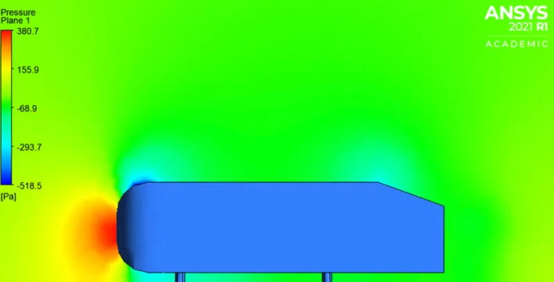
Pressure contour
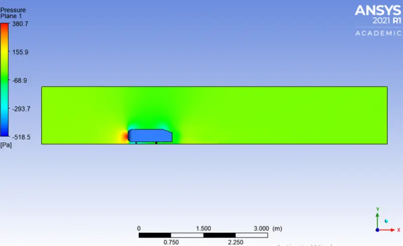
Wake region
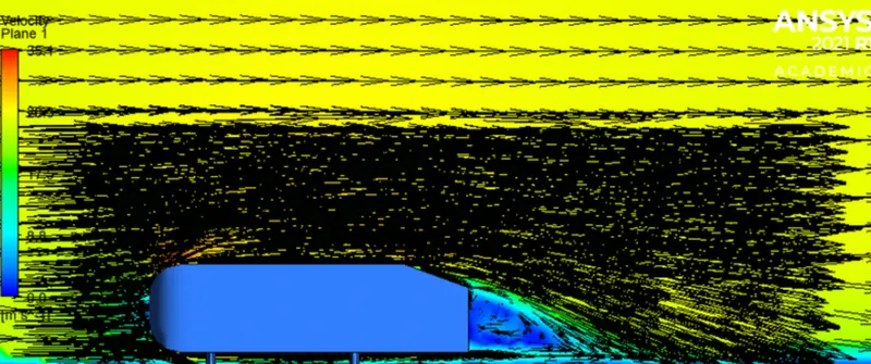
The vector plot showing the wake region
Drag coefficient 0.38361
Lift coefficient 0.30305
Case 2(b): Second refinement
Turbulence model: `k-omega` `SST`.
The multizone was used for the second area. The number of element size for the outer enclosure is taken as `90` `mm` whereas the element size for the inner closure is taken as `45` `mm`. Face sizing was implemented for the pillars of Ahmed's body (`5mm`).
Inflation layer
First layer thickness: `3``mm`
Number of layers: `10`
Last layer thickness: `15.4793``mm`
Number of elements: `253152`
The value of y+ is around 207.
Residual plot
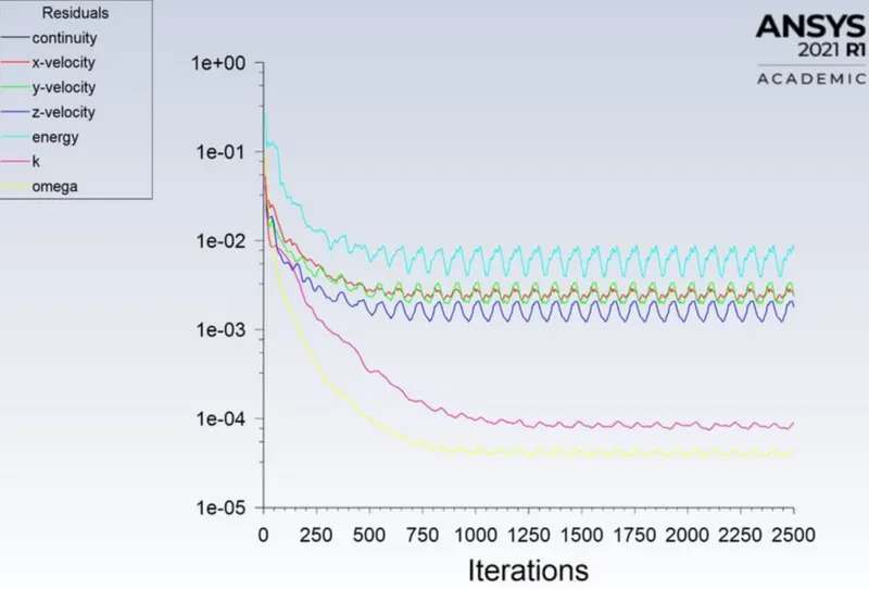
After 1600 iterations the same repeating trends are observed.
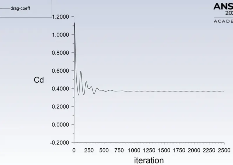
Drag coefficient
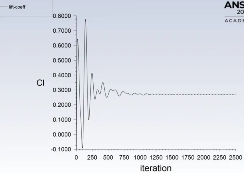
Lift coefficient
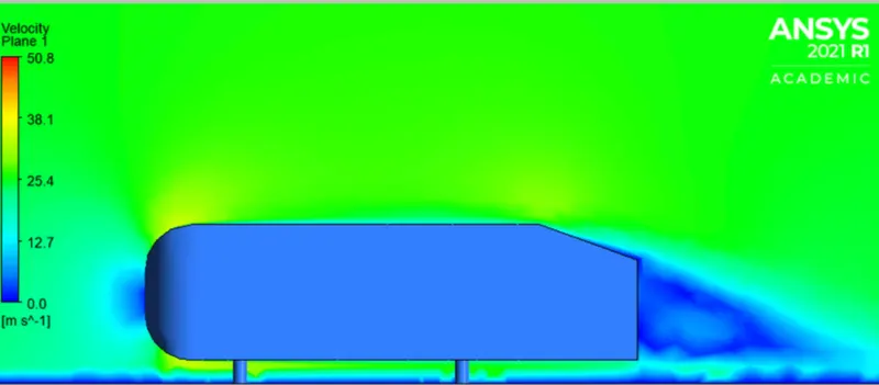
Velocity contour
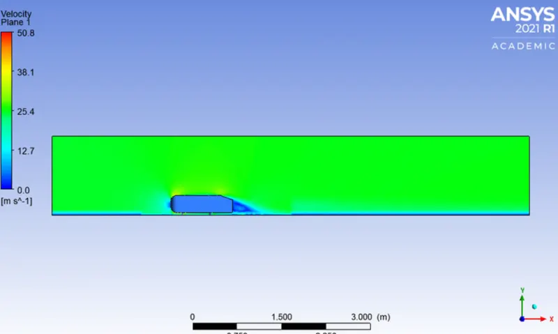
Wake region
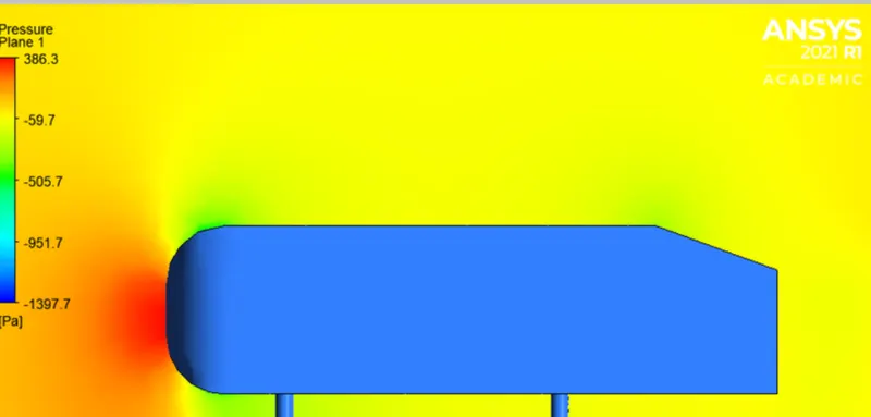
Pressure contour
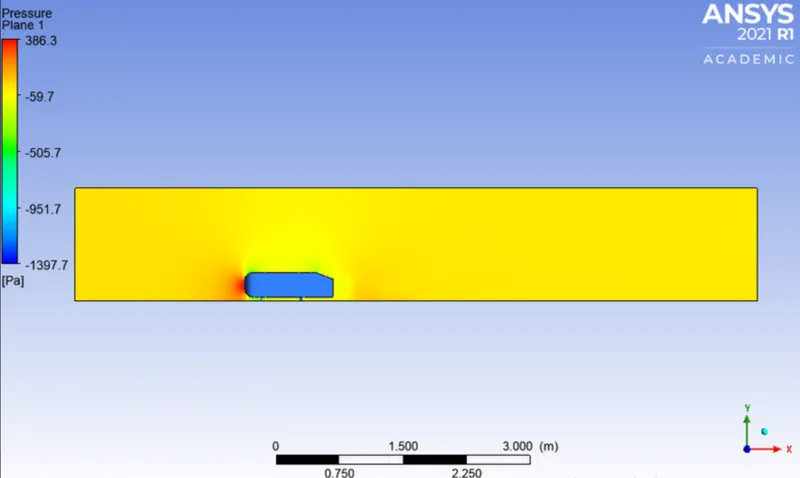
Wake region
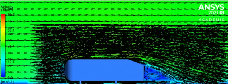
Vector plot showing the wake region
Drag coefficient 0.3512
Lift coefficient 0.2889
Case 2(c): Third refinement
Turbulence model: `k-omega` `SST`.
Element size in the first enclosure: `80mm`
Element size in the second enclosure: `40mm`
Element size of the bottom leg of Ahmed body: `5mm`
The size of the inflation layer: `10`
First layer thickness: `0.15mm`
Last layer thickness: `0.77mm`
Number of elements: `348448`
Residual plot
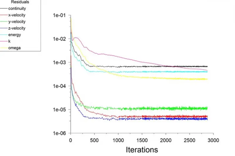
After 1200 iteration the repeating trends are observed.
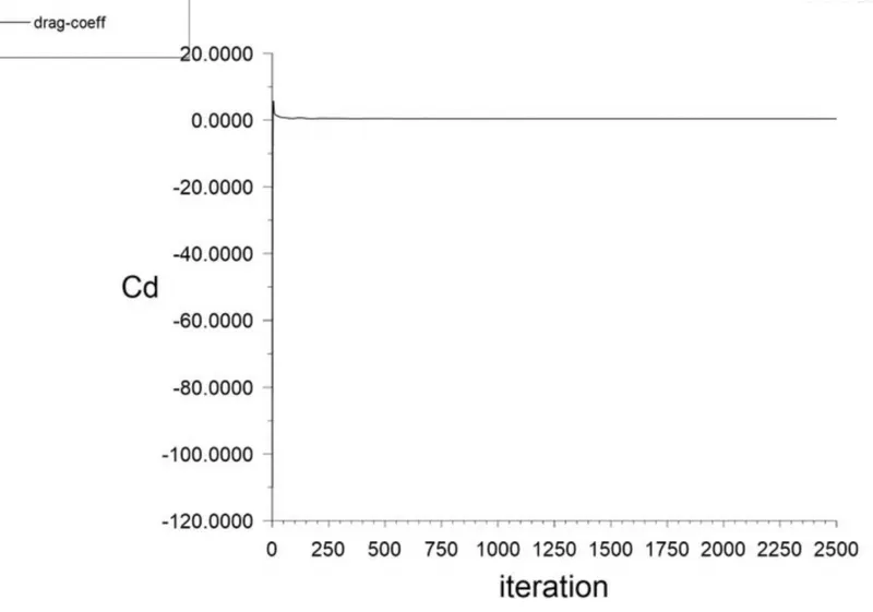
Drag coefficient plot
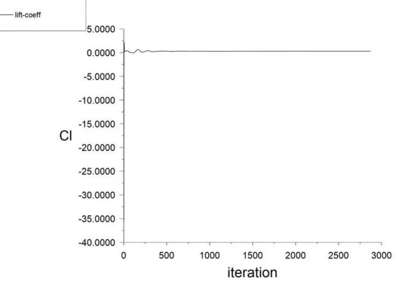
Lift coefficient plot
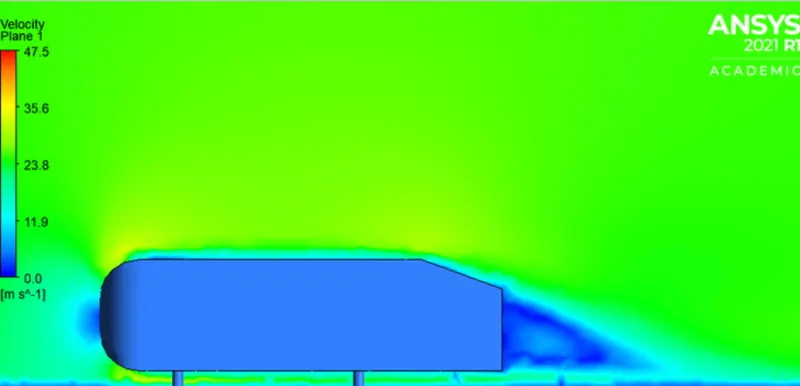
Velocity contour
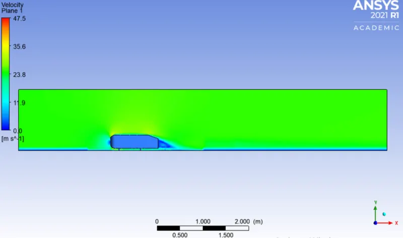
Wake region
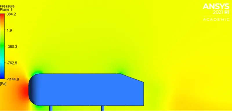
Pressure contour
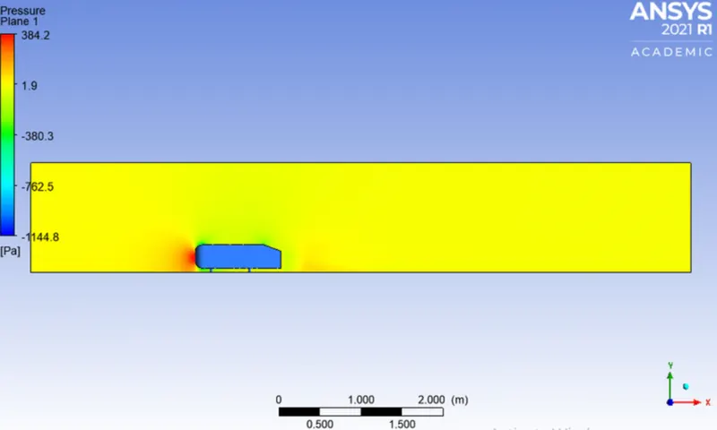
Wake region
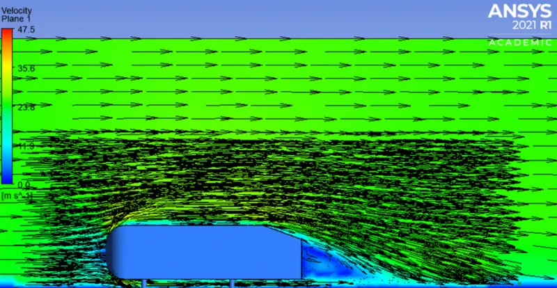
Vector plot near the wake region
Drag coefficient 0.3498
Lift coefficient 0.2884
Demonstration of grid independence test
Comparison of all cases
Steady-state, turbulent flow, Density-based, Fluid Material-Air
|
Grid Independence Test |
Turbulence-model |
Number of elements |
Lift-Coefficient |
Drag-Coefficient |
|
Baseline mesh |
`k-epsilon` |
`83781` |
`0.5865` |
`0.7253` |
|
First refinement |
`k-omega``SST` |
`192628` |
`0.3030` |
`0.3836` |
|
Second refinement |
`k-omega``SST` |
`253152` |
`0.2889` |
`0.3512` |
|
Third refinement |
`k-omega``SST` |
`348448` |
`0.2884` |
`0.3498` |
It can be inferred that the imitation of the experimental result is obtained during the second refinement. Thus, the grid independence test saves a lot of computational time and convergence can be achieved by using smaller cell sizes for calculation.
Conclusion
It can be inferred that the grid independence test is performed to know the smaller cell size for convergence.
Apart from mesh refinement, convergence depends on the Y+ value, inflation layer, it is advisable to use `k-omega``SST` as the turbulence value because it calculates the values well near the wall.
As the setup is refined drag coefficient, lift coefficient decreases.
Y+ plays an important role in determining the value of drag.
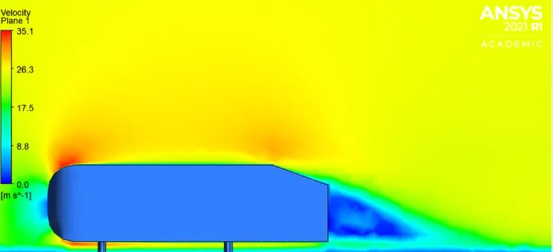
The negative pressure in the wake region is primarily because there is no flow in that region. This can be further attributed to various factors such as separation and recirculation which is evident from the vector plot near the wake region.
The point of separation occurs at the rear end of the vehicle, the separation occurs beyond this point where it can be observed that the flow recirculates and attaches it to the boundary layer.