Week 3 - External flow simulation over an Ahmed body.

External Flow Simulation over an Ahmed Body

Aim :- 1.To describe Ahmed body and it's imporatance.

2.To explain the reason for the negative pressure in the wake region.

3.To explain the significance of point of separation.

4.To plot the drag-coeffcient,velocity and pressure contour plots.

(By running the simulation for the inlet velocity of 25m/sec.)

Introduction and Theory :-

Ahmed body :- Ahmed body is a generic car body(a simplified car model).The airflow around the ahmed body captures the essential flow features around an automobile and was first defined and characterized in the experimental work of 'Ahmed'(name of a scientist).Althouh it has a very simple shape, ahmed body allows us to capture the characteristic features that are relevant to bodies in the automobile industry. This model is also used to describe the turbulent flow field around a car like geometry.

Importance of Ahmed body:- The drag coefficient quantifies the resistance of an object in a fluid environment.It is not an absolute constant for a body's shape because it varies with the speed and direction of flow,object shape and size and the density and the viscosity of the fluid.The lower the drag coefficient of an object,the less aerodynamic or hydrodynamic drag occurs.Incase of a car,the lower the drag coefficient the more efficient the car is.Working on Ahmed body helps a lot to decrease the drag coefficient.

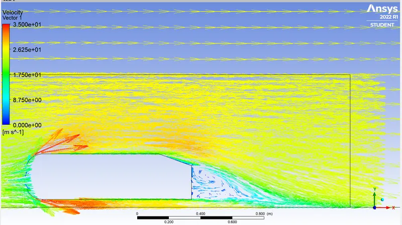
Wake region & the point of separation :- The flow region which presents the major contribution of a car's drag, and which poses severe problems to numerical predictions and experimental studies as well, is the wake region behind the car.The location at which the flow separates determines the size of the separation zone, and consequently the drag force.A more exact simulation of the wake flow and of the separation process are essential for the correctness of the drag predictions.

YPlus :- Wall functions are useful in telling the solver how toapproach the solution near a wall. These are used to predict near-wall results accurately even at coarse grids.Before going into wall functions there are two terms to understand.The first is the boundary layer and the second is the y+.

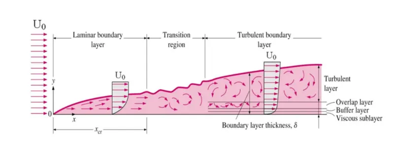
The image attached shows the boundary layer development.We first start in the laminar region,then transition to the turbulent region.Near the wall due to the viscous forces,the velocity is dragged to zero and as the boundary layer develops,the velocity will reach free-stream velocity.This is termed as the no-slip condition.

We can use the no-slip condition if we know the flow is completely laminar.This would mean that we are resolving the flow in the laminar region whatever the grid size.This,however doen't hold if the flow is turbulent.Turbulent flows have a smaller laminar region near the wall and if we are to resolve the gradients at such a small region,we'd need a very small grid size.

This is where the y+plus value comes in handy.The Y+ value is a non-dimensional term that can be used to understand how coarse or fine our grid is.This can then be used to determine if wall functions need to be used or not.From the image attached above, we need to either be in the viscous sub-layer or turbulent region.If we were in the viscous sub-layer,that would mean a y+ of less than 10 and if we were in the turbulent region,it would mean a y+ of greater than 30.

• y+ = y*Ut/v where y is the distance from the wall and Ut is the frictional velocity.

• Ut = √(Tw/ρ) where Tw is the wall shear stress, Tw = 1/2(Cf*ρ*U^2) , ρ is density, Cf is the skin friction coefficient

• Cf = 0.0576 * Re^(-1/5)
• Using the y+ the way in which velocity is calculated changes.

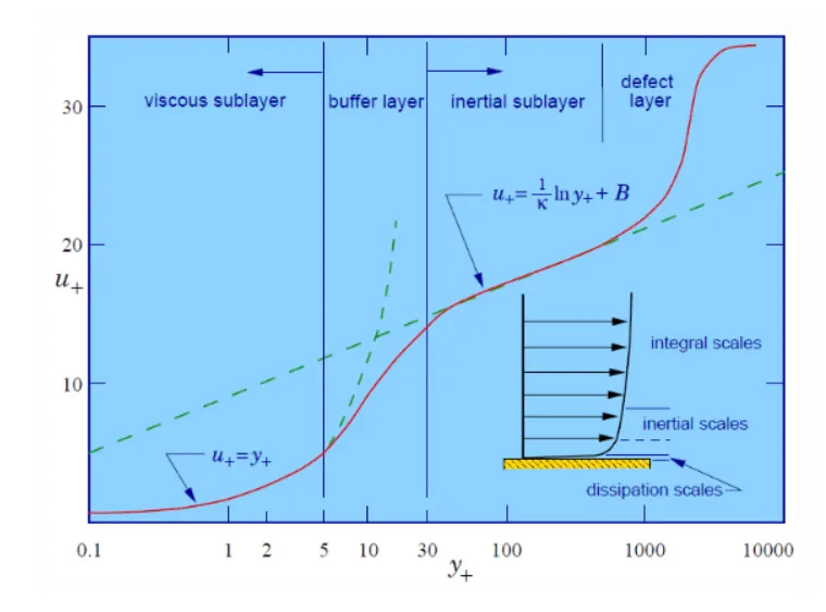
The significance of y+ :- The y+ value denotes where in the y+ vs u+ curve we are with respect to the cell size.It is undesirable to have a cell size that leads to a y+ of between 10 to 30 since the modelling of flow transitioning from laminar to turbulent is not easy and is still being researched.Due to this fact it is better to have a y+ of less than 10 meaning we'd at the laminar region or have a y+ of greater than 30 where we can go with a wall function and still acheive results.The y+value can be used as a marker based on which we can decide on the base grid size and make a decision based on the computing power as to whether the grid needs to be refined further or coarsened.

Density based solver/pressure based solver:-

The pressure based solver traditionally has been used for incompressible and mildly compressible flows.The density based approach on the other hand was originally designed for high-speed compressible flows.Both approaches are now applicable to a broad range of flows(from incompressible to highly compressible).

Geometry :-

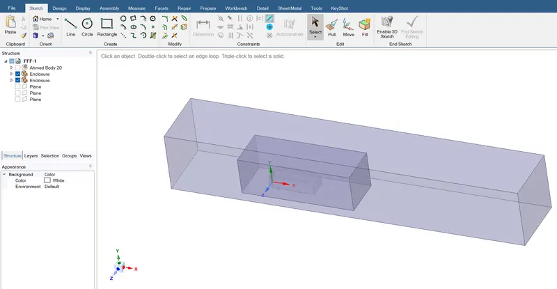
1. Import the Ahmed body model to spaceclaim to prepare the geometry.
2. Suppress the ahmed body as we don't want to mesh inside the body.
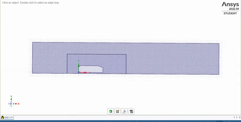
3. Create the rectangular enclosures around the ahmed body for meshing.Inner enclosure for more specified meshing.
4. Check the interference for the enclosures and insert the x,y,z planes.
5. Close the geometry and now spaceclaim will autosave the geometry.

Meshing :-

1. Insert method and use multizone method for meshing (Hexagonal meshing)

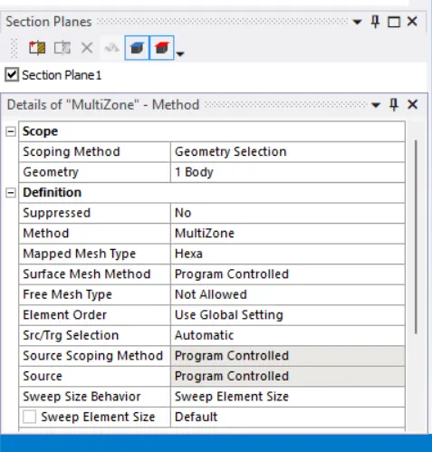
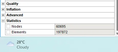
2.Element size 0.1m,since there is an abrupt change in the walls of ahmed body,we have used inflation with growth rate of 1.2 and 5 layers around the ahmed body's wall.

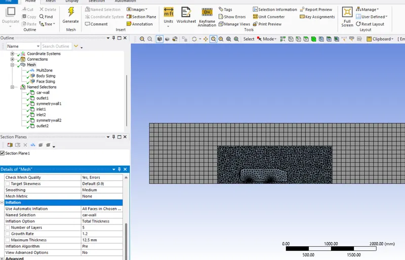
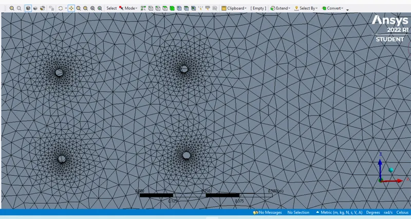
3.Refined mesh :-

Should get finer meshing where the ahmed wheels should look like a circle instead of polygons. Select the face sizing method and select the 4 faces and reduce the element size from 50 mm to 5 mm.

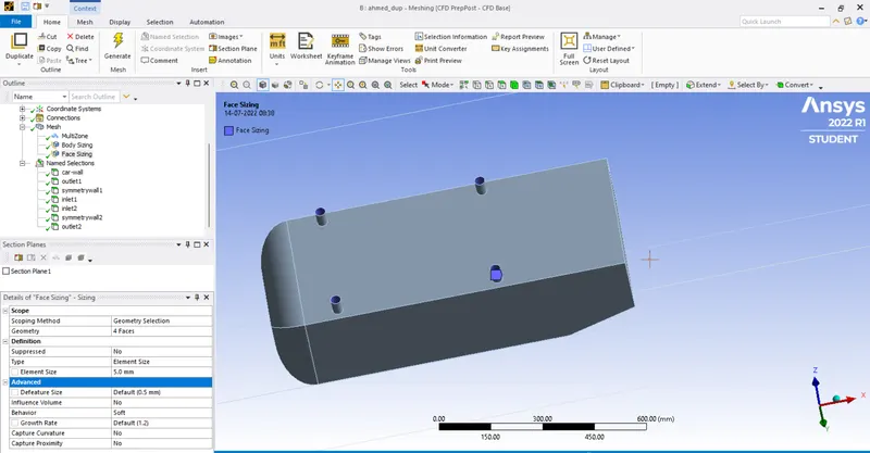
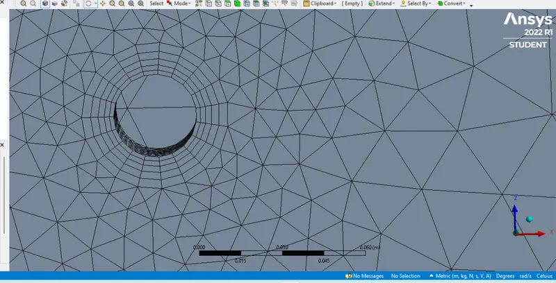
4.Using Box-select tool create an enclosure around the ahmed body and name it as car-wall and give the required namings for other parts.

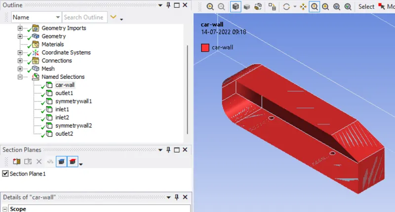
5.Now close the meshing and open Ansys Fluent setup.(also give the required naming for the various selections)

Setup:-

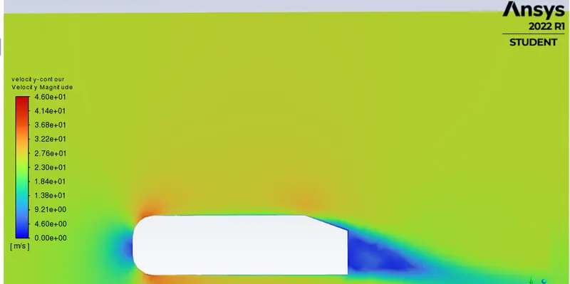
We are using a steady state solver to run the simulation and to capture the lift and drag coefficients.We capture the wake region behind the ahmed body inorder to investigate why the flow is separated and why we have negative pressure in the wake region.We use 'k-omega' equation model as it suits best for the study near the wall where adverse pressure gradient is developed..(k-epsilon is best suited for flow away from the wall)

Density based solver or pressure based solver(Choosing type of solver) :-

Speed of air at inlet = 25m/s , Speed of sound = 344m/s, Mach number = 25/344 = 0.07, since the mach number is less than 0.3 we will be using the pressure based solver as it is an incompressible flow.Re = 1759696 , therefore the flow is turbulent.

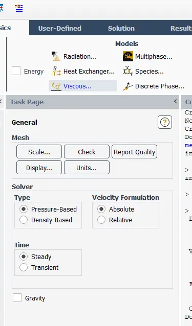
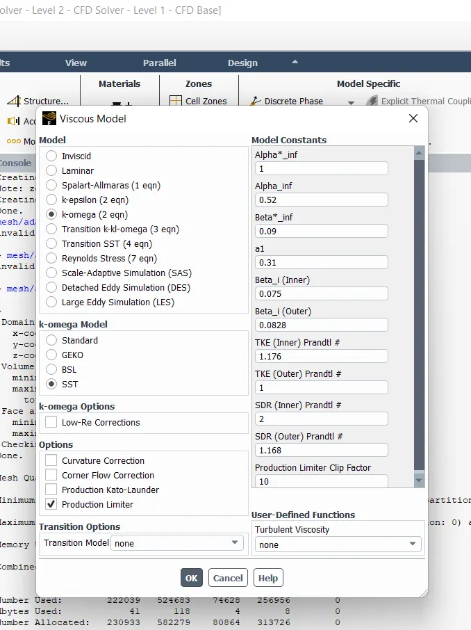
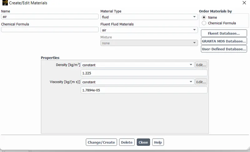
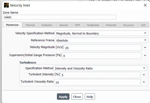
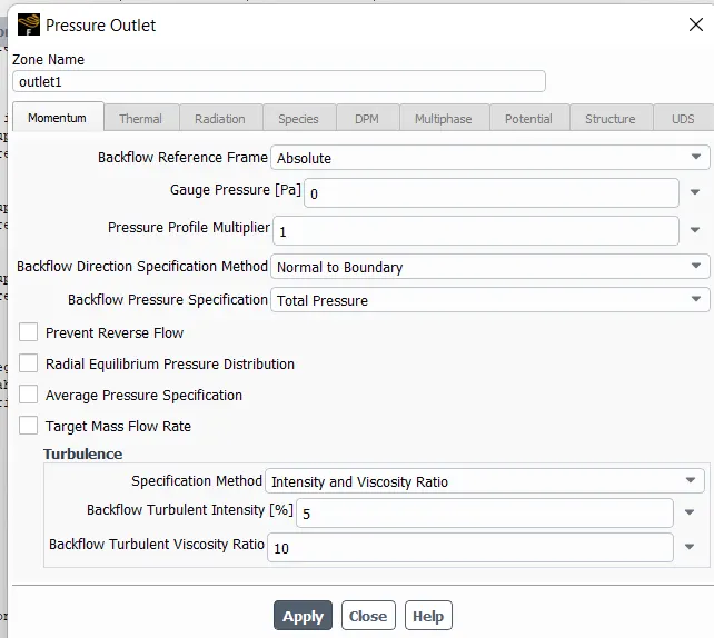
• We had run the simulation for 500 iterations and started the calculations.

Results :-

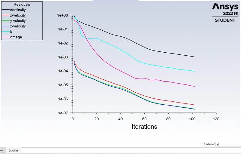
Scaled residuals :-

Drag coefficient :-

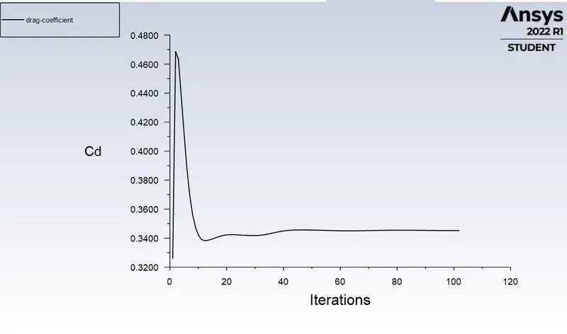
Drag coefficient value :- After 102 iterations, the solution is converged.And we obtained the drag coefficient = 0.3452 according to the experimental data it should be 0.33, so the error percentage is 1% which is less.

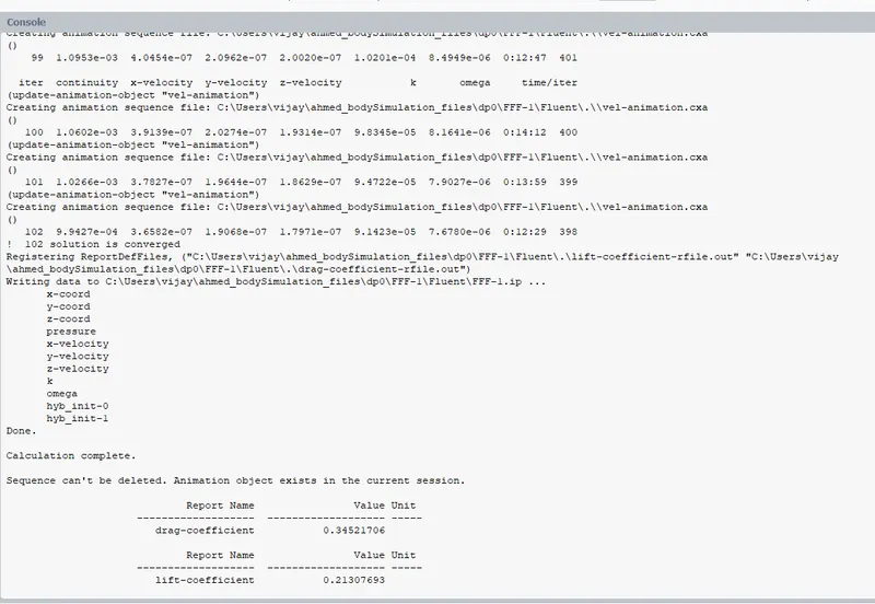
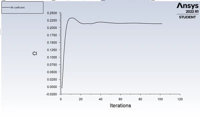
Lift coefficient :-

Velocity plot:-

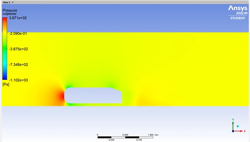
Pressure contour :-

Vector plot:-

Grid Independency test :-

Case1:-

Inner enclosure mesh size = 50mm

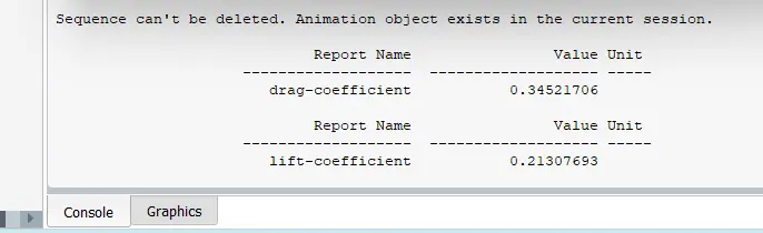
Drag coefficient = 0.3452 , Lift coefficient = 0.2130

Case2 :-

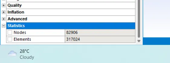
Inner enclosure mesh size = 40mm

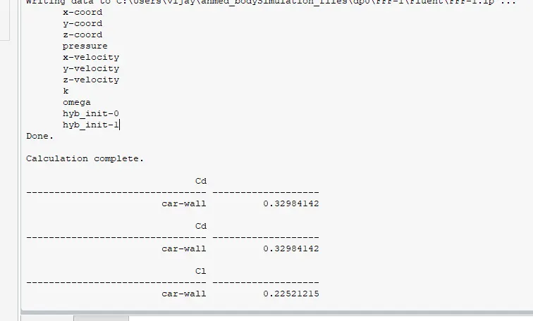
Drag coefficient = 0.3298(more accurate), Lift coefficient = 0.2252

Conclusion :- We successfully simulated the Ahmed body in various cases and calculated drag coefficient and lift coefficient values with very less error percentage.We had run the simulation with an inlet velocity of 25m/s.

Reason for negative pressure in the wake region :- The pressure inside the wake region remains low as the flow separates and a net pressure force(pressure drag) is produced.Due to the production of pressure drag being produced from flow separation,the pressure in the wake region is low.This causes the vaccum.