Week 3 - External flow simulation over an Ahmed body.

Aim: The aerodynamic behavior of an Ahmed body is numerically investigated in the present work. Commercial fluent software is used for CFD simulation using a turbulent model. Grid dependency test is performed to validate the result against the experimental data. Computational drag and lift fairly agrees with the numerical simulation.

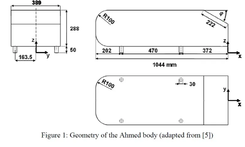
Theory: The Ahmed body was first created by S.R Ahmed in his research “Some salient features of the time –Averaged Ground vehicle wake” In 1984 since then, it has become a benchmark for aerodynamic simulation tool. The simple geometry shape has a length of 1.044 meters, height of 0.288 meters and a width of 0.389 meters. It also has 0.5 meters cylindrical legs attached to the body ad rear surface has a slant that falls off at 40 degrees. The Ahmed body is a bench mark model widely used in the automotive industry for validating simulation tools. The Ahmed body is simple in shape, enough to model while maintaining car like geometry features.

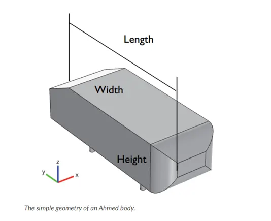
Modelling Air flow over an Ahmed Body:

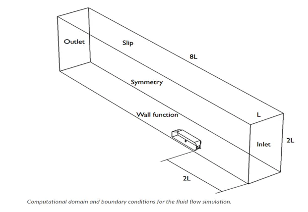
In the airflow over an Ahmed body verification model, Our Ahmed body has a 25-degree slant and is placed in the following domain measuring 8.352-by-2.088-by-2.088 meters. To compute the flow field.

The front of the body is placed at a distance of 2car length (2L) from the inlet flow. To reduce the computational cost, a symmetry plane is introduced to model half of the model.

The flow for this model is turbulent, which is based on the Reynolds number determined by the body length and inlet velocity. The simulation solves for the turbulent kinetic energy in addition to the velocity field, for this simulation, We need a larger mesh size than what is usually common to resolve the turbulent flow .More specifically we use a finer mesh downstream of the model to capture the wake zone.

The flow for the model is turbulent, which is based on the Reynolds number determined by the body length and inlet velocity. The simulation solves for the turbulent kinetic energy and dissipation in addition to the velocity and pressure.

The total drag coefficient of the Ahmed body is the key measurement for the simulation. It is made up of measurements for the pressure coefficients in the front, slant and base of the body as well as the body skin friction . In the result of our simulation, the total drag is very well predicted but the individual measurements deviate from the experimental results in varying amounts.

A few different factors cause these deviation in data . For the front and roof of the body , wall functions used in the simulation are not effective at predicting the flow transitions observed in the experiments.

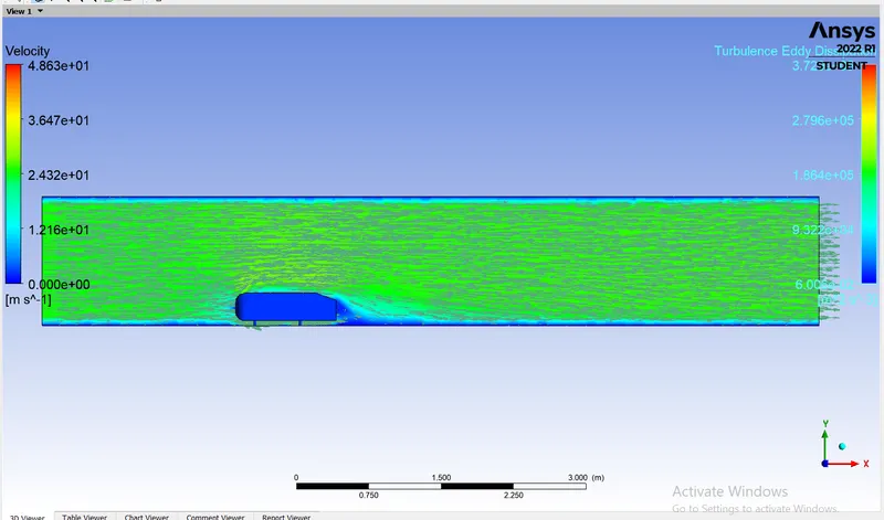
In the term of deviation the slant coefficient data , we see the flow along the slant shown by streamlines in the figure below. The thickness of these streamlines is determined by turbulent kinetic energy.

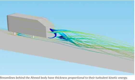
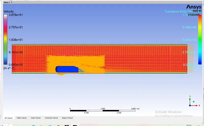
In the experimental data , these lines shows that the flow along the slant is attached almost everywhere and that there are two small re circulation zones behind the base.in the simulation results , This effect is captured but the extent of the recirculation zones are over-predicted.

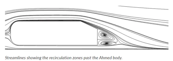
The pressure drag for the slant coefficient is very sensitive to the exact shape and location of the recirculation regions , which accounts for the deviation in measurements.

Although the data has quantitative differences , it is qualitatively equal to experimental results because the total drag coefficient are so close.There may be deviating details in the smaller data but the simulation still captures the major features of the flow over an Ahmed body. The simulation is more than adequate for calculating the overall drag coefficient .

Problem Statement:

1. Describe Ahmed body and its importance.
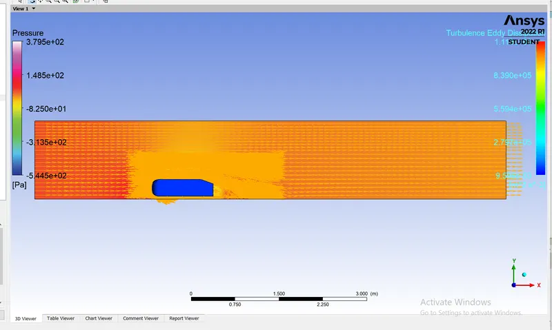
2. Explain the reason for the negative pressure in the wake region.
3. Explain the significance of the point of separation.

Expected results:

1. Velocity and Pressure Contours.
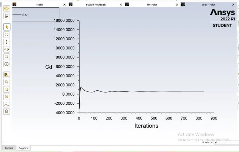
2. The drag coefficient plot for a refined case ( For velocity of 25 m/sec , The drag coefficient should be around 0.33).
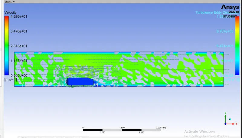
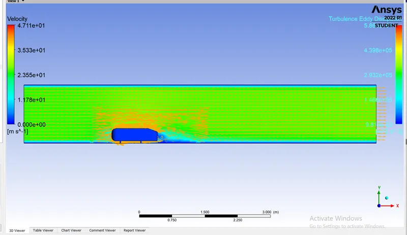
3. The vector plot clearly showing the wake region.
4. Perform the grid independency test and provide the values of drag and lift with each case.

GEOMETRICAL DIMENSIONS OF AHMED BODY:

Different views of Ahmed body with dimensions is shown below.

Problem solving with modelling approach:

Meshing Methodology:

Geometry case setup:

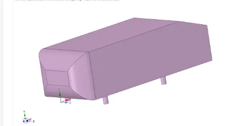
The model is loaded in ansys space claim from stp file format.

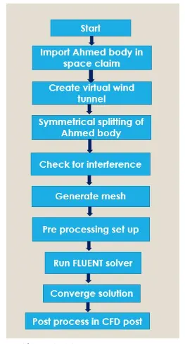
The Ahmed body is enclosed by a virtual wind tunnel created by enclosure option in prepare physics tool box, unchecked the symmetric option.

Create the inner box using the enclosure option.

Select a plane perpendicular to the Ahmed body to check the cross section view.

Checking for interface , Separate the outer closure from the inner box and also the Ahmed body from the inner box.

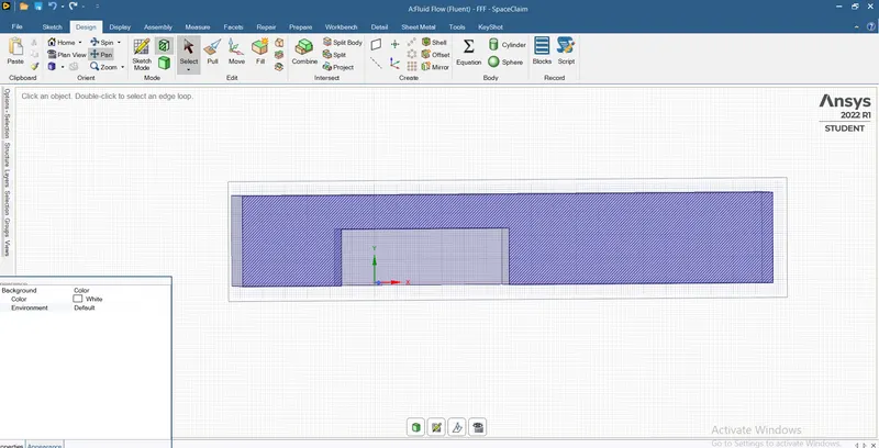
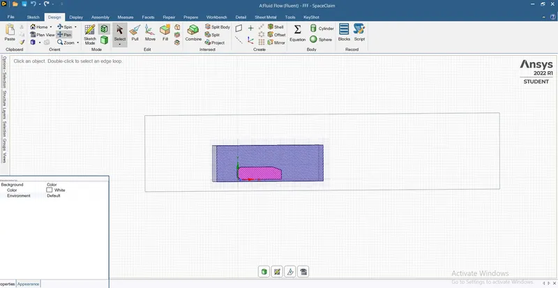
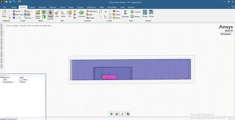
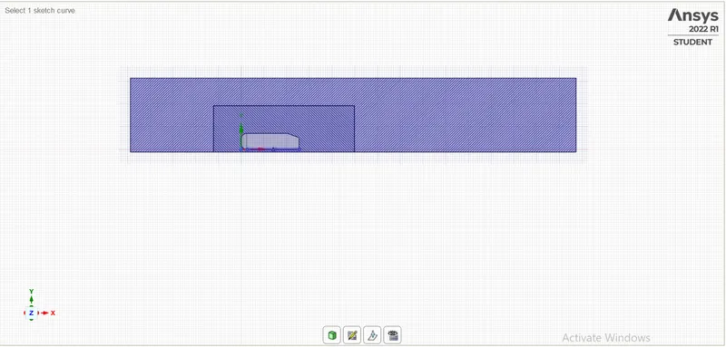
After interface checking , click on split body command to split the Ahmed body and the enclosure in one half and inner enclosure with Ahmed body and Surpressing Ahmed body

Meshing Geometry setup:

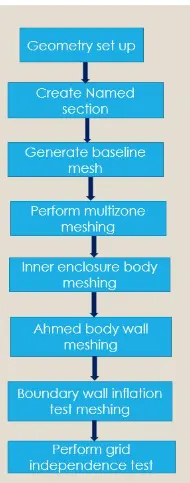
Baseline mesh:

* Open the meshing console.

* click on mesh option on the left side of work tree diagram.

* Click on generate mesh.

* A general mesh pattern will be created.

* Create section plane on one half of the geometry.

* inlet

* Outlet

*Symmetry

* Car wall

*Click on the mesh option on the left hand side of work free diagram.

* A general mesh will be created.

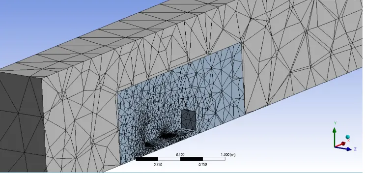
* To refine mesh, click on automatic methods, Select the outer wind tunnel box, Go to the methods and select multiple zone options. Click on mesh generate.

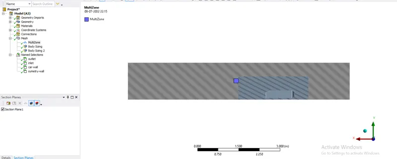
* To give required size, Click on mesh and give the required mesh size.

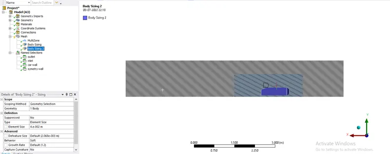
* To refine the inner box click on Sizing option by right click on mesh , Select the inner box. Give the required mesh.

* To define the Ahmed body part, Hide all the faces other than the car wall.

* Use box select tool to select the faces of the car wall.

* Give the required size of mesh , Generate mesh.

* Now to refine the cylindrical Pillars of Ahmed body , click on sizing, Select face preparation , use single select tool Select the cylindrical portion.

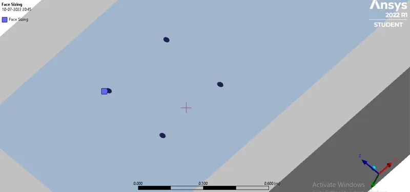
* Giving the size click on generate mesh.

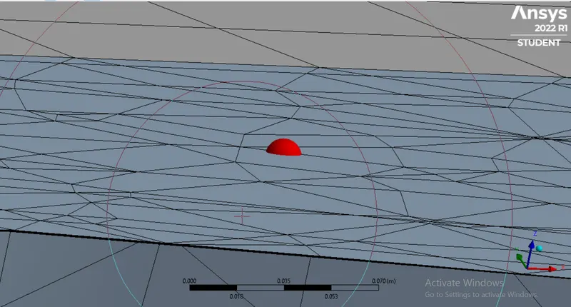
* Now go to mesh , Click on inflation ,Select geometry from named section , Choose car wall < Give the no of layers and total thickness based on Y+ generate mesh.

Setting up per-processing Physics:

* Select density - based solver

* Viscous model is selected as k-epsilon model.

* Setting up boundary conditions.

* Set up inlet conditions as 25 m/s.

* set up the reference values.

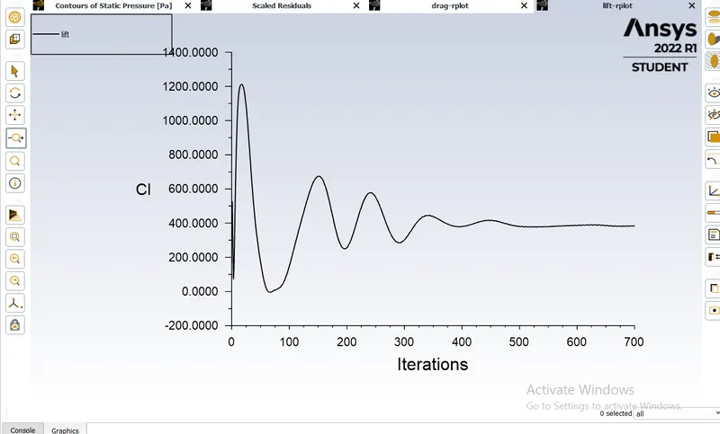
* Create report definition of drag and lift plot.

* Create a plane using point and normal method.

* Set up initialization by choosing hybrid initialization method.

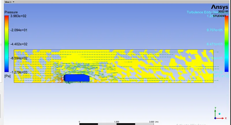
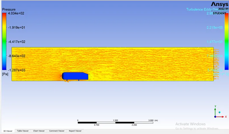
* Create pressure and velocity contour plot across the cut plane.

* Create animation plot of velocity and pressure contour.

* Set the no of iterations to run the fluent solver.

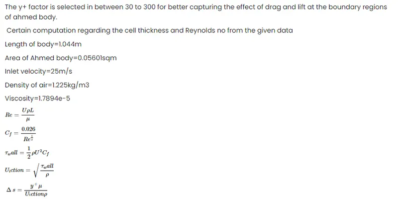
COMPUTATING FIRST CELL THICKNESS LAYER FROM Y+ FACTOR:

POST PROCESSING PHYSISCS FOR BASE LINE MESH:

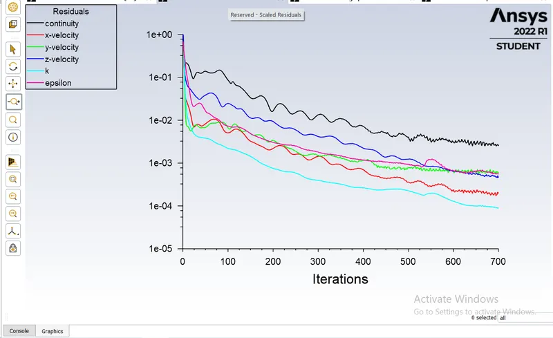
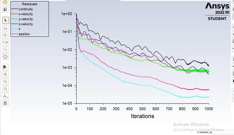
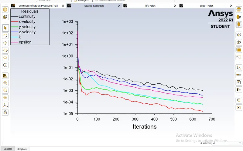
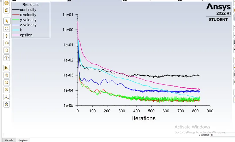
* Iteration convergence.

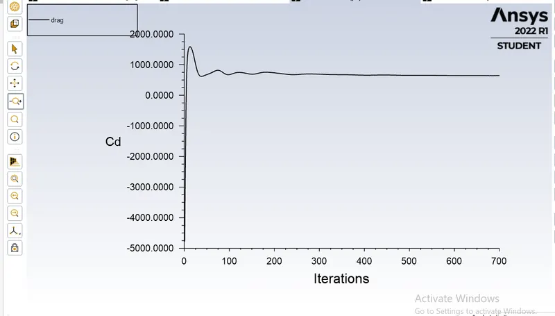
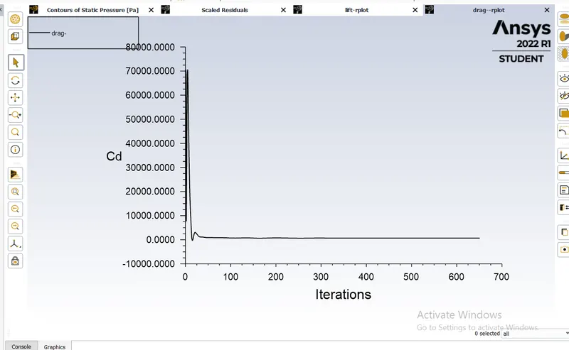
* Drag plot

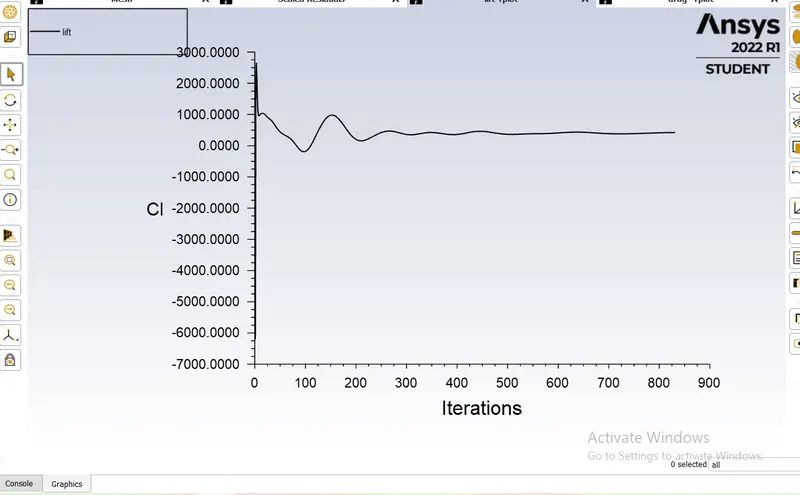
* Lift Plot

POST PROCESSING VELOCITY VECTOR PLOT:

POST PROCESSING PRESSURE VECTOR PLOT:

Grid dependence test:

In this study we have set about 4 cases , by refining the mesh at different sizes and also at different Y+ values The table below shows the difference cases considered for the grid dependence test.

Outer wind tunnel	Inner box closure	Ahmed Body	Nodes	Elements
120mm	50mm	5	105967	342535
100mm	45mm	5	127396	367265
80mm	40mm	5	152441	372135
60mm	35mm	5	175241	456021

The table below shows at different Y+ set up taken.

Y+	1st cell thickness	Total thickness	No of layers	cd	ci	Drag error(%)
70	1.028mm	3.069mm	7	0.0329	0.1987	15.97
100	1.46mm	7.533mm	10	0.380	0.2308	13.32
150	2.196mm	19.579mm	13	0.274	0.2735	12.54
200	2.928mm	37.605mm	15	0.37	0.2576	10.98

POST PROCESSING PHYSICS FOR GRID INDEPENDENCE TEST REFINED MESH:

CASE1:

* Outer wind tunnel :120mm

* Inner enclosure box:50mm

* Ahmed body : 5mm

* Y+=70

MESH SYMMETRY CASE:

Iteration convergence:

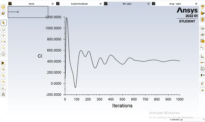
L plot:

Drag plot:

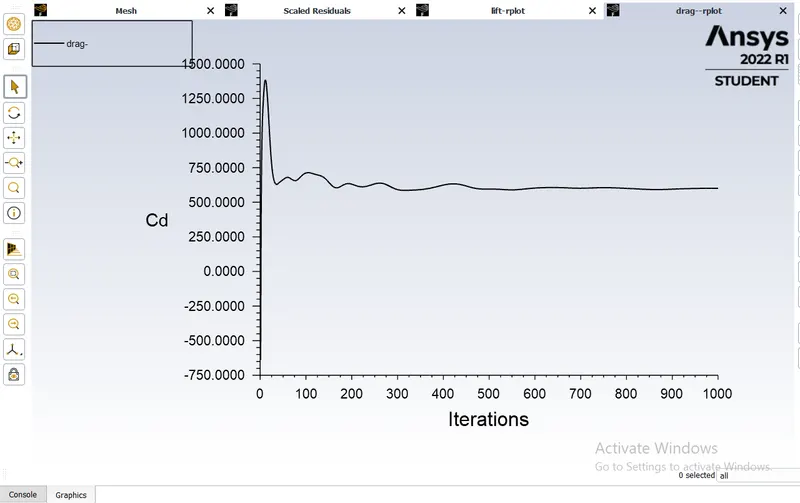
COMPUTED DRAG AND LIFT VALUES:

* POST PROCESSING VELOCITY VECTOR PLOT

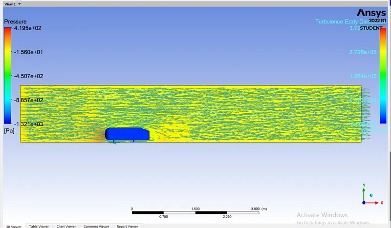
* POST PROCESSING PRESSURE VECTOR PLOT

CASE2:

* Outer wind tunnel :100mm

* Inner enclosure box:45mm

* Ahmed body : 5mm

* Y+=100

MESH SYMMETRY CASE:

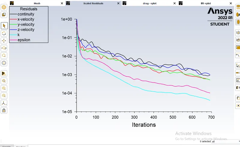
Iteration convergence:

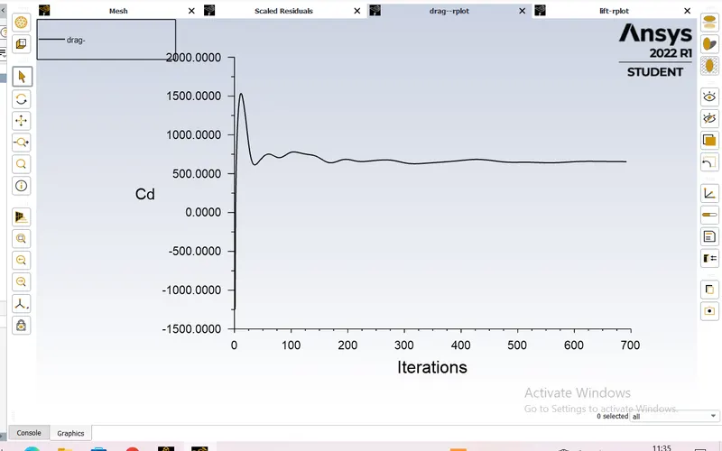
Drag plot:

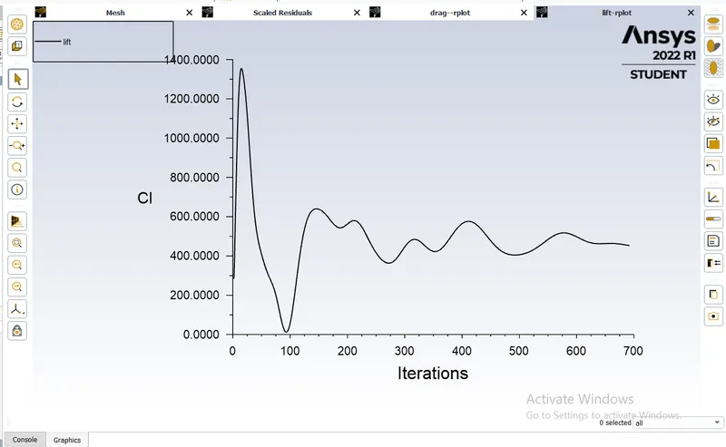
Lift plot:

COMPUTED DRAG AND LIFT VALUES:

* POST PROCESSING VELOCITY VECTOR PLOT

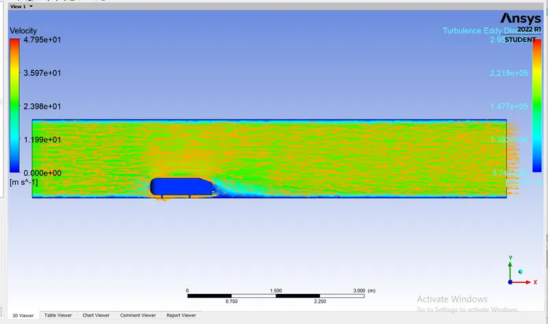
* POST PROCESSING PRESSURE VECTOR PLOT

CASE3:

* Outer wind tunnel :80mm

* Inner enclosure box:40mm

* Ahmed body : 5mm

* Y+=150

MESH SYMMETRY CASE:

Iteration convergence:

Drag plot:

Lift plot:

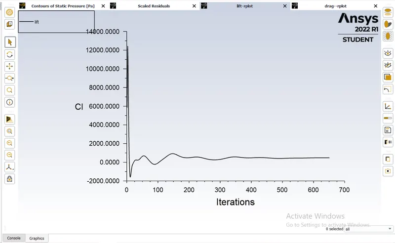
COMPUTED DRAG AND LIFT VALUES:

* POST PROCESSING PRESSURE VECTOR PLOT

* POST PROCESSING VELOCITY VECTOR PLOT

CASE4:

* Outer wind tunnel :60mm

* Inner enclosure box:35mm

* Ahmed body : 5mm

* Y+=200

MESH SYMMETRY CASE:

Iteration convergence:

Drag plot:

Lift plot:

COMPUTED DRAG AND LIFT VALUES:

* POST PROCESSING VELOCITY VECTOR PLOT

* POST PROCESSING PRESSURE VECTOR PLOT

NAVIGATE PRESSURE GRADIENT

When fluid velocity increases , the pressure decreases . The wake region is formed due to adverse pressure in the rear end causes the boundary layer to separate out from the body. The wall shear stress and velocity becomes Zero and wake up formation starts.These wakes are nothing but small vortices that create negative pressure. These create circulation of velocity and induces drag forces.

POINT OF SEPERATION:

Separation occurs due to an adverse pressure gradient encountered as the flow expands , Causing an extended region of separated flow .The part of the flow that separates the recirculating flow through the central region is called the dividing stream line.The point where the dividing stream line attaches to the wall again is called the reattachment point . As the flow goes farther downstream it eventually achieves an equilibrium state and has no reverse flow.When the boundary layer separates it remnants from the shear layer and the presence of a separated flow region between the shear layer and surface modifies the outside potential flow and pressure field. In this case of airfoils The pressure field modification results in an increase in pressure drag.

CONCLUSION:

*From running a baseline simulation , the post CFD results gave inaccurate results at the region of mesh overlapping.

* The grid independence test shows best results close to the experimental data.with refining the mesh size with Y+ factor , The error is significantly reduced .

* The Y+ is chosen in between a stable range to give a correct prediction of velocity and pressure contour plots.

* The flow separation and appearance of vortices gets more prominent as Y+ is increased. As seen in baseline meshing no wake formation is captured properly , on refining the mesh , the flow is captured properly.