Drop test

Aim: The objective of this assignment is to prepare a model and run a simulation of a drop-test for the provided mesh inputs of a cell phone and a floor.

Theory: The basic idea here is not to get correct results, but to put together keywords and boundary conditions so that we can run the simulation without running into problems and get a rough idea on what we would be doing in complex projects. Thus, we would need bare minimum keycards to run this simulation.

Every input file is made up of keywords that shape our simulation. A keyword is something that defines everything that a solver would need and understand to provide us meaningful results. Given below is a list of keyword that is necessary for LS-Dyna.

• *Keyword: Consider this as the opening statement of the coding that the solver would understand. Every input file must start with this keyword. If we prepare a model from scratch then we don’t even have to create this keyword as this is saved by default while saving the model.
• *Control: This keyword provides the setting that we need to control the simulation. For example, *Control_Contact, *Control_Termination, and *Control_Accuracy just to name a few. There are numerous control cards present in LS-Dyna, however, *Control_termination is mandatory to define as this will tell the solver how long a user wants his/her simulation to run.
• *Node, *Part, *Element: When working professionally, we would be given mesh data which would be fed into the solver. Thus, these three keywords are made by the solver once it gets relevant data, so again we do not have to define this keycard manually. Even if we make a mesh from in the Pre-Post, these keywords will be defined again as the solver will take it directly.
• *Section: This is one keyword that is very important to get approximate results. It defines what our part looks like. For example, we usually mesh sheet-metal components in 2D mesh ignoring its thickness. The section keyword lets us communicate with the solver that this component has x thickness so consider this while computing the results. Even if the component is solid, we have to define this keyword to tell the solver that it is a solid section.
• *Material: This keyword defines the material for the part. LS-Dyna offers a wide range of options to choose the materials from. We have to enter the material properties to define a material through this card.
• *Boundary: This entity allows us to define the constraints that a part might have. For example, in some cases, we might need our part to move only in the x-direction so we can constrain its motion in other directions. This entity will not allow the elements to move in the constrained direction, thus compelling them to stick to the motion that a user desires.
• *Database: This keyword allows users to ask for outputs from the solver that it has after running the simulation. It is mandatory to request a Binary d3plot as output as it will have animation of the simulation and other plots like energy, stress, strain, displacement, etc.
• *Initial: This keyword is required from this model to define the initial velocity with which a cell phone will fall to the ground. Apart from velocity, we can also give initial displacement or acceleration to the model.
• *End: The input file ends with this keyword.

Procedure:

Step-1: Load the input file in the LS-Prepost and delete the unnecessary part. We can see there is a shell element and a Brick element for the floor, so we can delete either one of them according to our wish. I have deleted brick elements and worked with shell elements.

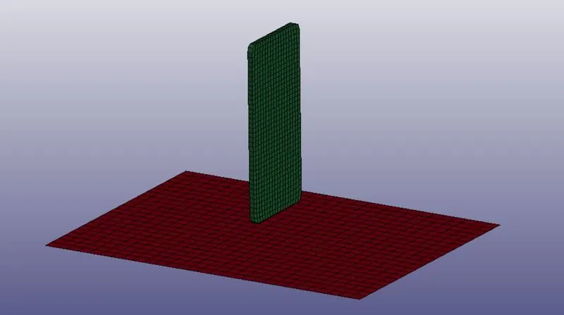
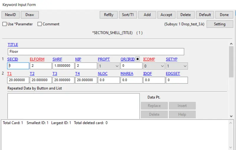
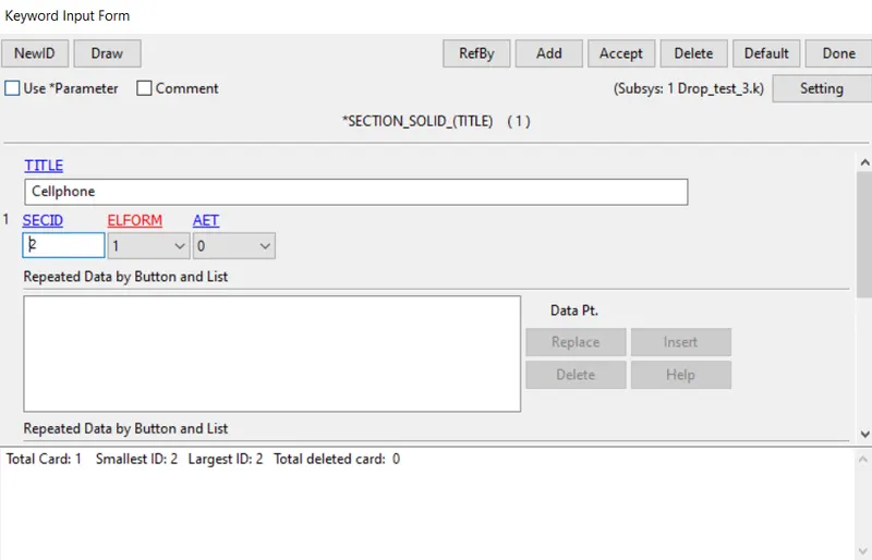
Step-2: Create a section keyword. Here we have created a shell section for the floor with an arbitrary thickness, and solid elements for the Cell phone.

• Go to Model and part> keyword manager> All
• Scroll down to Section> Shell
• Enter section Id, title, and thickness.
• Hit accept and done.
• Scroll down to Section> Solid
• Enter section id and hit accept and done.

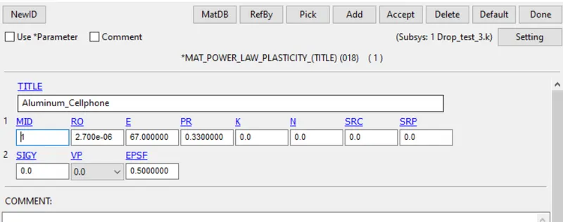
Step-3: Create Material keywords. Here we will create two material cards, aluminum for cell phones and rigid for the floor.

• Go Model and part> keyword manager> All
• Scroll down to Material> Power-law elasticity (018)
• Enter the title as aluminum, section id, density, young’s modulus, Poisson's ratio, and elastic failure strain.
• Hit accept and enter.
• Now, scroll down to Material> Rigids
• Enter the title as the floor, section id, and material properties.
• Hit accept and enter.

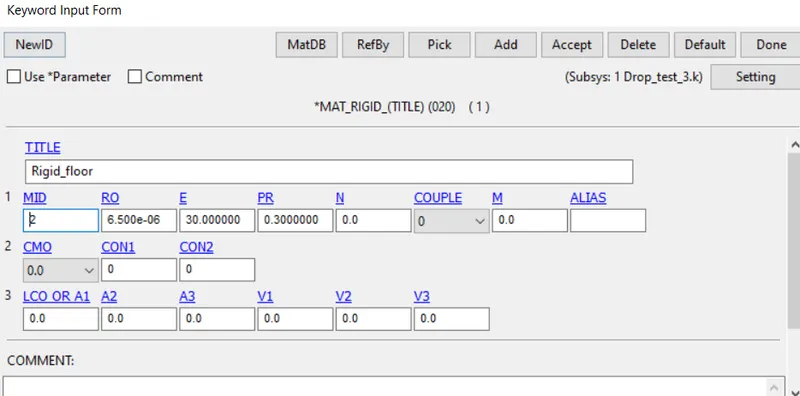
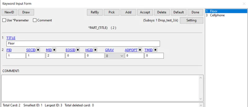
Step-4: Assign the material card and section card to the respective parts. Here we will tell the solver which card is associated with which part.

• Go Model and part> keyword manager> Model
• Go to part. Here we can see two parts. Rename them as cell-phone and floor.
• Now, go to a cell phone (vertical brick elements) and assign sections and material according to the title.
• Repeat the same procedure for the floor

One thing to note here is the use of the title. If we use the title effectively, we will not get confused when we are working with numerous parts in one model. Thus, always give a title such that it can be understood by a new person working on your model.

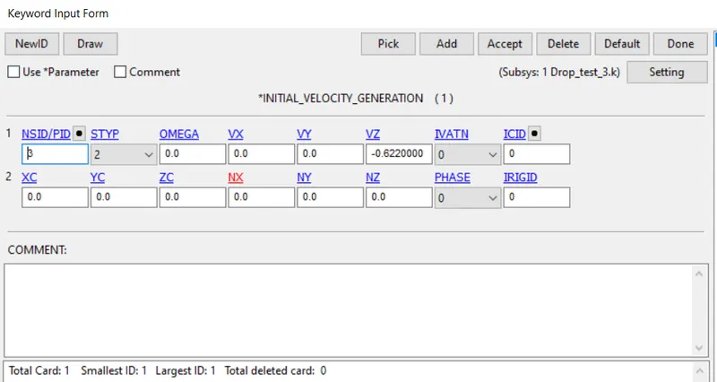
Step-5: Applying initial velocity. We are considering a free-fall condition in which the phone will be under the influence of gravity only. Thus, we can do the necessary calculations to get the velocity with which it would be falling. Using the equation of motion, v^2=u^2+2gs and considering the unit system as Kg, mm, ms we get the value of velocity as 0.662mm/ms.

• Go Model and part> keyword manager> All
• Scroll down to Initial> Velocity generation
• Enter Styp as 2 and then select the cell phone. Now, enter the value in Vz as -0.662 as it will be going in the negative z-direction.
• Hit accept and done.

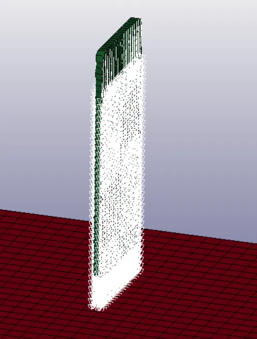
Step-6: Defining contact interfaces. Here we will be defining master and slave nodes for the model. Usually, master nodes are stiffer than the slave nodes, and we are interested in studying the slave nodes. Thus, a cell phone is a slave and the floor is the master here.

• Go Model and part> keyword manager> All
• Scroll down to Contact> Automatic Surface to surface
• Enter id, title, and STYP as 3 for both master and slave.
• Now, select the master as the floor part and the Slave as the cell phone part. Hit accept and enter.
• Now, scroll down to contact> Automatic single surface
• Enter id, title, and define self-contact for cell phone part. Here master and slave nodes will be the same part.
• Hit accept and done.

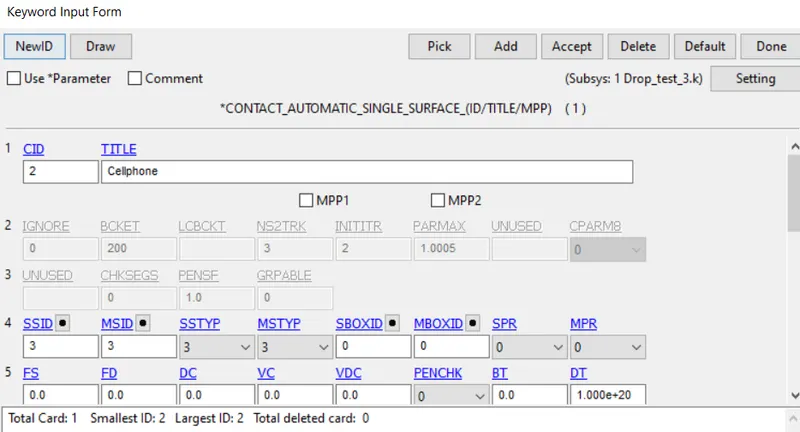
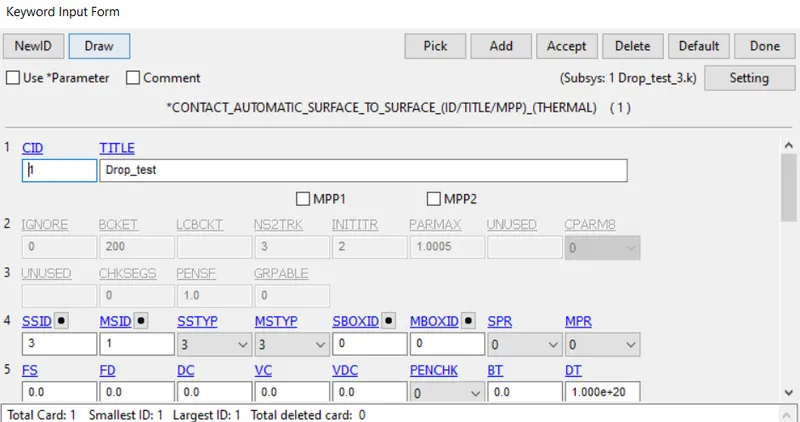
Step-7: Control termination. Here we will define the total simulation time.

• Go Model and part> keyword manager> All
• Scroll down to Control> Termination
• Enter Endtim value as 20ms. As I have used 20mm thickness, the distance between the cell phone and the floor is reduced and there is no sense in running the simulation for a longer time.
• Hit accept and done.

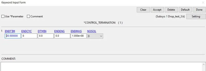
Step-8: Requesting output. We will only request for d3plot output.

• Go Model and part> keyword manager> All
• Scroll down to Database> Binary d3plot
• Dt as 0.1. Now the solver will write the output file every 0.1ms.
• Hit accept and done.

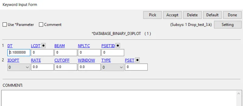
Step-9: Boundary condition. Here we do not need to fix the floor as it is already rigid. It will not let anything penetrate it, and neither will it move from its position. The defining boundary condition for the floor would result in warnings as we would over define the model.

Step-10: Model checker. It is good to run a model checker as it will display errors and warnings that will not let the solver run the simulation.

• In the keyword manager, hit model checker
• In the new window, go to keywords
• Run the checker
• Solve the errors or warnings, if any.

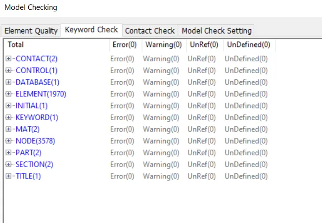
Step-11: Run the analysis.

• Save the keyword
• Open LS-run
• Load the model in this window
• Hit run and let the solver compute the solution

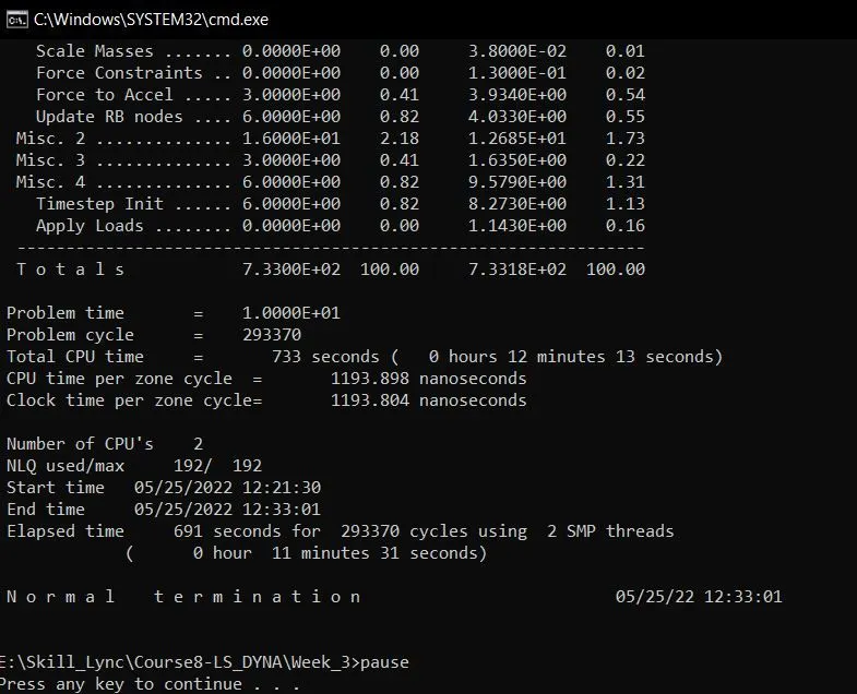
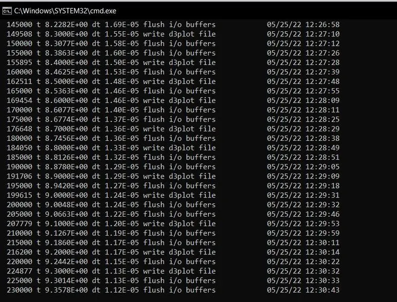
Step-12: Check the animation and plot graphs.

• Once the animation is complete, the open the binary plot in LS-prepost
• Here we can see the animation of the drop test
• In addition, we can check stress, strain, and other quantities
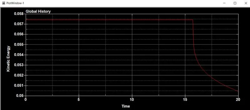
• Further, we can plot those quantities curves with respect to time.

Graphs:

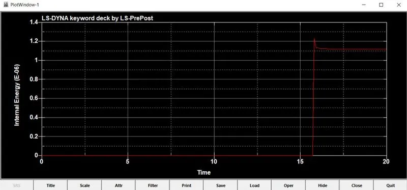
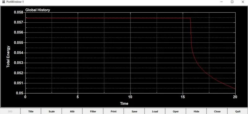
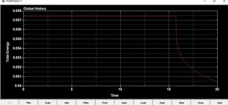
Conclusion: Through this assignment, I have learned to set up and run a basic simulation which has made me comfortable with the software and laid a foundation for more complex simulations.