Getting familiar with the ADVISOR Tool

AIM:

To use the ADVISOR tool and simulate:

1. The EV_defaults_in file in FTP (Federal Test Procedure) driving cycle with cargo mass as 500 kg and other default conditions.
2. The same simulation with increased battery capacity.
3. The PRIUS_Jpn_defaults_in file for gradeability test.

OBJECTIVE:

The objective of the project is to get familiar & learn the ADVISOR tool, its working & uses and analyse the effect of time and speed on the gradeability of the vehicle.

MODEL SETUP:

1.

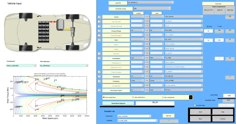
This is the model setup with default conditions we have for EV_defaults_in. The energy storage (battery) is of lead-acid type and is ESS_PB25 spec. The number of modules connected is 25 and the nominal voltage output of this storage is 308 V. The storage weighs 275 kg. The motor is MC_AC75 spec which produces 75kW of power, works at an efficiency of 92% and weighs 91 kg. A manual transmission is used which weighs 50kg. Here, we add a cargo mass (payload) of 500 kg.

After clicking on Continue, we get a different window where we can select/create the driving cycle, no. of cycles, carryout acceleration & gradability tests, apply auxilliary electrical loads. We select the FTP driving cycle and have 1 cycle.

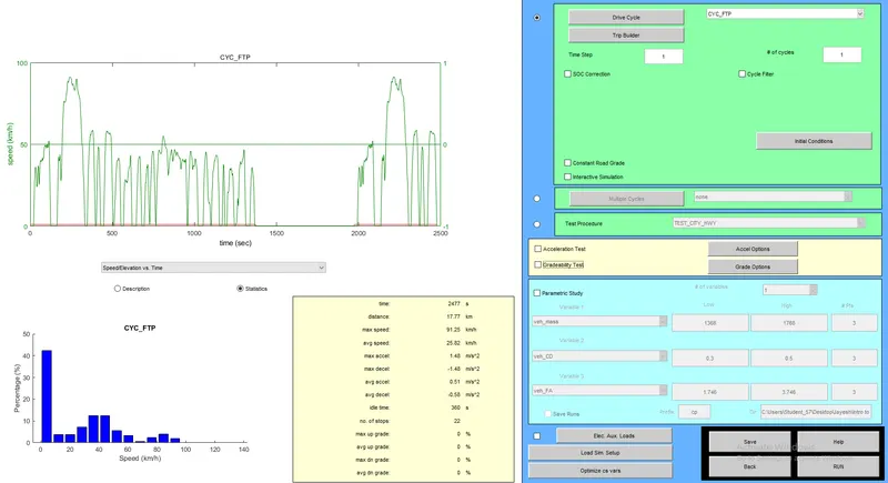
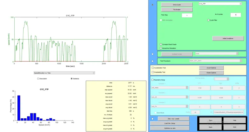
Since the distance covered in one FTP driving cycle is only 17.77 km, we increase the number of cycles.

3.

Here we have the Toyota Prius Japan model and we carryout simulation for the gradability test. We vary the speed & time by keeping one of the value constant to see their effect on the gradability of the vehicle.

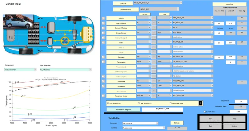
First, the time is kept constant at 10 seconds and the speed (mph) is increased.

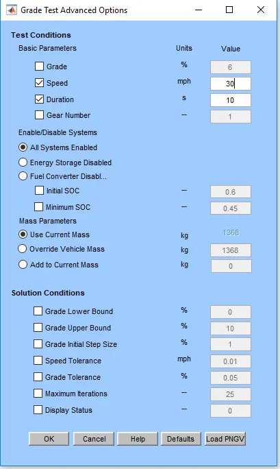
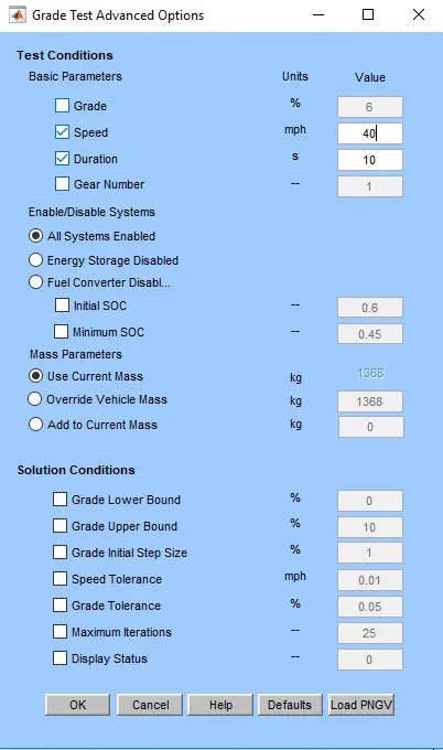
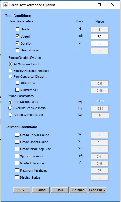
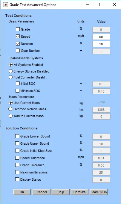
Then the speed is kept constant at 40 mph and the time (seconds) is varied.

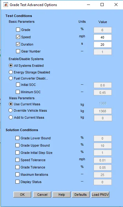
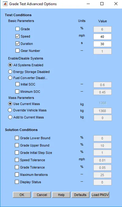
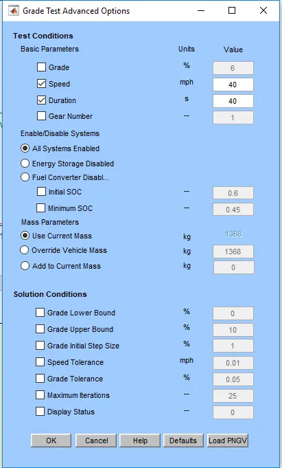
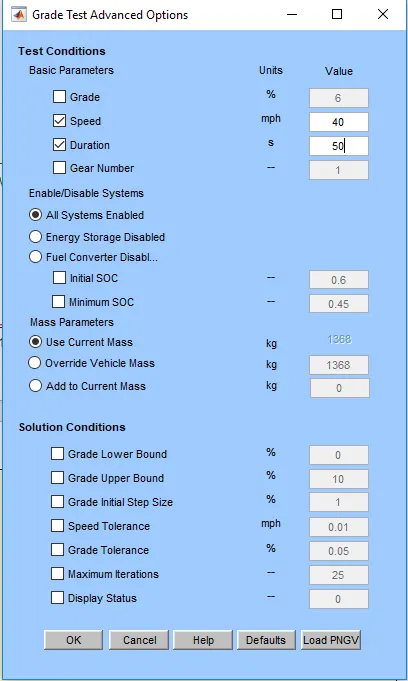
This way we keep the time constant and increase the speed to make a study and then keep the speed constant and increase the time to analyse the effect of speed and time on the gradeability of the vehicle.

EXPLANATION & RESULTS:

1. For the first case, we simulate the EV_defaults_in with all default conditions with the addition of cargo mass as 500 kg. Since the total distance travelled in one FTP (Federal Test Procedure) drive cycle is 17.77 km, we carryout the simulation for multiple driving cycles to see if we can cover 45 km.

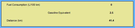
Here we can see that eventhough the total distance covered is more than 45 km, we were able to cover only 41.4 km. This can be seen with other parameters such as battery state of charge (SOC), current output from battery and motor torque,etc.

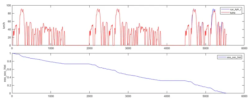
Here, the SOC of the battery has reached zero, meaning the battery has drained completely. This is the SOC when the distance covered is 41.4 km.

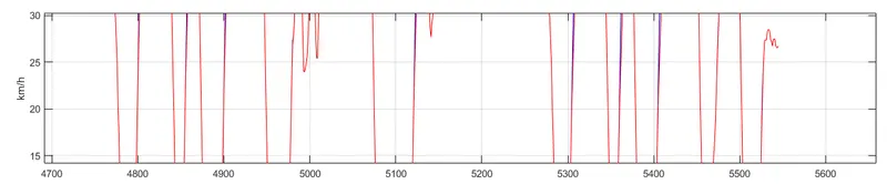
This is the actual plot of the driving cycle with the speed of the vehicle. Since the battery power is drained, the vehicle has stopped abruptly.

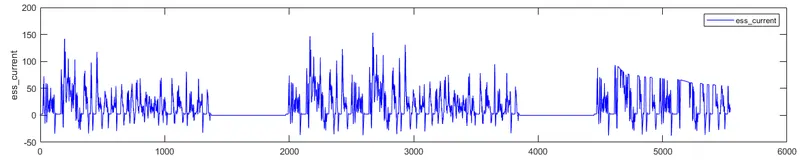
The above plot is the current output from the energy source (battery). We can see that the current supply is zero after 5000 seconds have passed. Further zooming the current plot and comparing it with the motor torque,

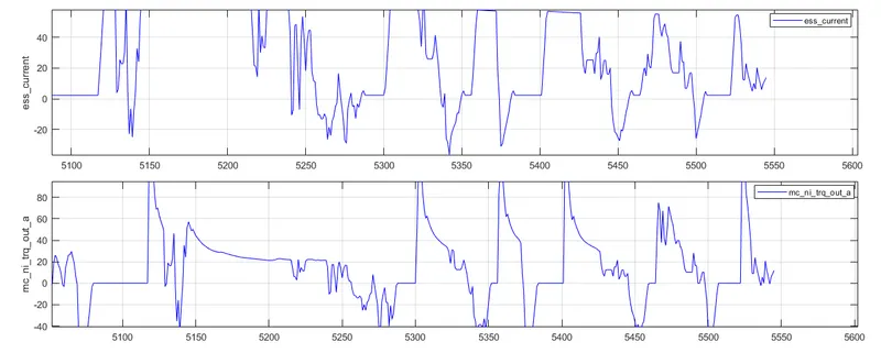
we can see that the current from the energy source and motor torque output stop at around 5550 seconds time.

Also we have got a warning & error message that required distance is exceeded by EV range, which further confirms that the vehicle cannot cover 45 km distance with the given conditions.

2. To increase the battery capacity, we increase the number of modules in the battery to 35. By running the simulation again, we get the following results.

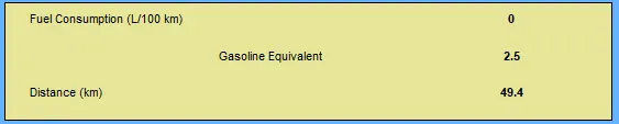
Here, we have covered the 45 km distance and reached upto 49.4 km.

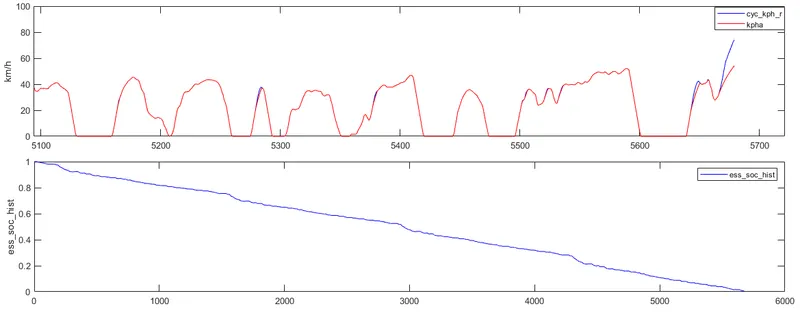
As in the previous case, the battery SOC has also reached zero but the time at which the battery is drained and the vehicle speed reduces is around 5680 seconds. Further comparing with the battery state of charge (SOC), current output from battery and motor torque,

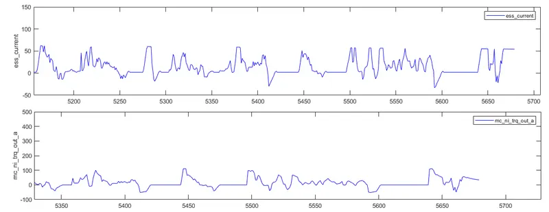
we can conclude that since the battery capacity has been increased, the range of the vehicle has also increased and the vehicle was able to run longer.

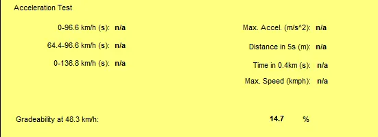
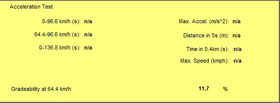
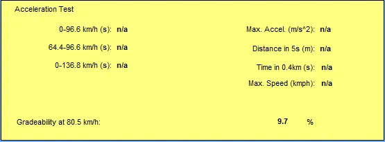
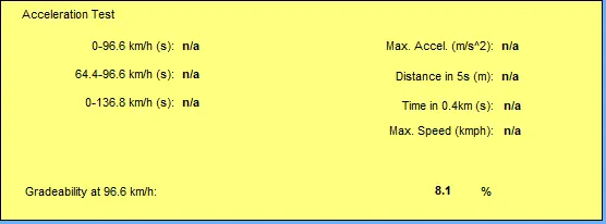
3. When the simulations are run, we get the results in a separate window. The results for speed varied vs constant time is as follows,

The results for constant speed vs varied time is as follows,

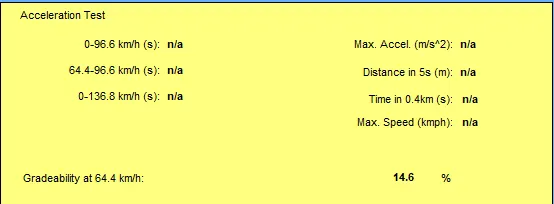
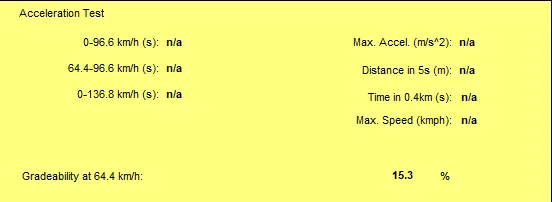
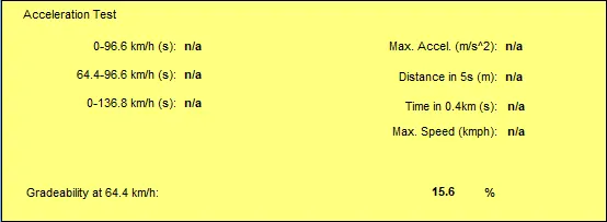
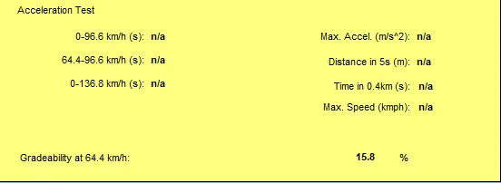
On comparing the results in a tablular form, we can analyse the effect of speed and time on the gradability of the vehicle.

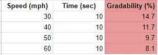
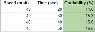
By looking at the above two tables, we can conclude that the gradability is good when there is a low speed and more time to climb a slope and the gradability is low when the speed is high & lesser time is provided. Lesser the time & more the speed means Lower the gradability. More the time & lesser the speed means Higher the gradability.

CONCLUSION:

Hence the learning of the ADVISOR tool and the effect of speed & time on the gradability has been analysed with the above project.