Week-3 Challenge: ADVISOR Tool

1)What is the ratio of hill climbing power required by fully loaded tata ultra truck to the half loaded one?

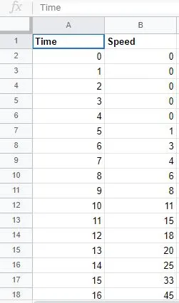
take a spreed sheet as A and B input 50 values

A as time and B as speed then enter values in time and the speed value will get.

2) A flyover is planned to be constructed on a national highway. Keeping in mind about the gradeability for trucks,how much can be the minimum length of the flyover, considering the minimum height at the summit should be 5.5 meters? State your assumptions.

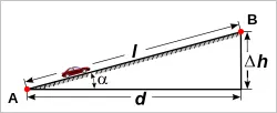
h= 5.5 m

αα=15o15o

L =hsin(α)hsin(α)

L=5.5sin(15o)5.5sin(15o)

L=21.250 m

d= l*(cos (alpha)`

d=21.250*(cos (15)`

d=20.526 m

3)Prepare a new drive cycle excel file having third column representing hill climbing angle corresponding to speed and time. Revise the model file “Driver_Glider.slx” such that it can calculate gradient force from drive cycle

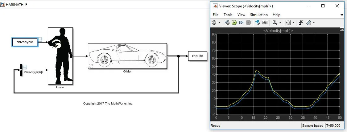
Glider subsystems:

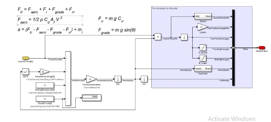
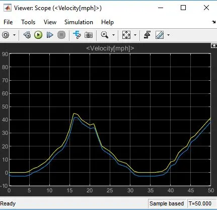
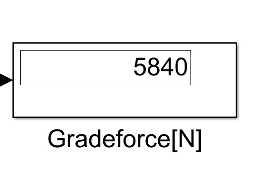
open glider lets shown that then select grade force(N) select main click the available option shown in the end as three dots more options are shown, click inclination angle then open that . the value changing option is shown their then input random number below 30 and select ok so the value is changed then continue run button tyhe graph is shown that value is changed as constant.

The inclination angle for this particular model is given as 20 degree.

GRAPH :

GRADE FORCE:

4) Model the WOT (Wide Open Throttle) response of GM EV1 car. Compare it with the official figures of the performance of a real vehicle. Prepare a table showing variation in acceleration time with 5% change in vehicle parameters.

• Features of GM EV 1
  Kerb_weight = 1400kg
  payload = 140kg
  Gross_weight =1540kg
  Gear_ratio = 11
  Tyre_radius = 0.30 m
  A=1.8 m^25%
• change in vehicle parameters.

Kerb_weight = 1400%kg
payload = 140%kg
Gross_weight =1463%kg
Gear_ratio =15.33
Tyre_radius = 0.265% m
A=1.71 %m^2
I=1540

• motor Characteristics
  till critical speed
  Tmax=140 Nm
  Angular_velocity = 733 Rad/s
  linear_velocity= 19.8 m/s
  Efficiency = 0.95

MATlab program to solve the equations using a time step of 0.1 sec

clear all
close all
clc

%Features of GM EV 1
Kerb_weight = 1400%kg
payload = 140%kg
Gross_weight =1540%kg
Gear_ratio = 11
Tyre_radius = 0.30% m
A=1.8 %m^2
%motor Characteristics
%till critical speed
Tmax=140 %Nm
Angular_velocity = 733 %Rad/s 
linear_velocity= 19.8 %m/s
Efficiency = 0.95
%above critical speed 
%T=2756/v

%GM Ev1 Acceleration
t=linspace(0,15,151); % 0 to 15 seconds, in 0.1 second steps
v1=zeros(1,151); % 151 readings of velocity
v2=zeros(1,151)
dT=0.1; % 0.1 second time step
% In this case there are three phases to the acceleration, as
% explained in the text.
for n=1:150
if v1(n)< 19.8
v1(n+1) = v1(n) + dT*(3.11 - (0.000137*(v1(n)^2)));
elseif v1(n) > 35.8 
% Controller stops any more speed increase
v1(n+1) = v1(n);
else
v1(n+1) = v1(n) + dT * ((62.1/v1(n)) - 0.046 - (0.000137*(v1(n)^2)));
end;
end;
v1=v1.*3.6; %convert to kph

%variation in acceleration time with 5% change in vehicle parameters.  
Kerb_weight = 1400%kg
payload = 140%kg
Gross_weight =1463%kg
Gear_ratio =15.33
Tyre_radius = 0.265% m
A=1.71 %m^2
I=1540
for n=1:150
if v2(n)< 19.8
v2(n+1) = v2(n) + dT*(4.9673 - (0.00018*(v2(n)^2)));
elseif v2(n) > 35.8 
% Controller stops any more speed increase
v2(n+1) = v2(n);
else
v2(n+1) = v2(n) + dT * ((62.92/v2(n)) - 0.04465 - (0.000131*(v2(n)^2)));
end;
end;
v2=v2.*3.6

plot(t,v1,'DisplayName','(WOT) acceleration of GM EV1 electric car' );
xlabel('Time/seconds');
ylabel('velocity/kph');

hold on

plot(t,v2,'DisplayName',' (WOT) acceleration of GM EV1 electric car with 5% change in vehicle parameters ');
xlabel('Time/seconds');
ylabel('velocity/kph');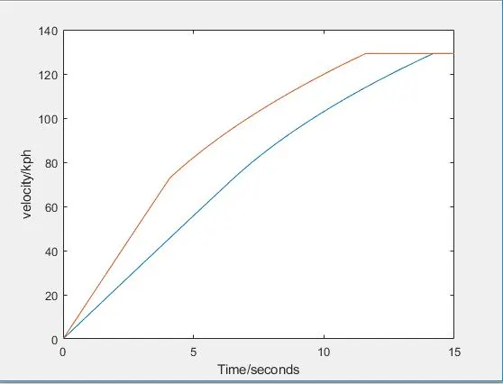

From the plot we can say that the reduction in vehicle parameters by 5% reduces the acceleration in time .